Introduction
If you are choosing betwixt a prima schema and a snowflake schema for a PostgreSQL analytics database, commencement pinch this rule: usage a prima schema erstwhile query velocity and ETL simplicity are your superior constraints, and usage a snowflake schema erstwhile retention efficiency, referential integrity, and often updated magnitude attributes matter more.
Both schemas instrumentality dimensional modeling for OLAP workloads. PostgreSQL supports some without extensions, and some tally connected DigitalOcean Managed PostgreSQL. If you are evaluating PostgreSQL against different database systems, the comparison of relational database guidance systems covers why PostgreSQL is commonly chosen for analytics usage cases.
The quality betwixt the 2 schemas is simply a trade-off betwixt denormalization and normalization successful the magnitude tables that situation your cardinal truth table. This tutorial walks done DDL examples for some patterns utilizing a accordant unit income scenario, compares EXPLAIN ANALYZE output for balanced queries, and covers indexing and configuration for analytics workloads connected managed PostgreSQL.
In this tutorial, you will study really to instrumentality prima and snowflake schemas successful PostgreSQL, measure their query capacity utilizing EXPLAIN ANALYZE, configure DigitalOcean Managed PostgreSQL for analytics workloads, and take betwixt the 2 patterns utilizing a repeatable determination framework.
Key Takeaways
- A prima schema denormalizes each magnitude attributes into level tables, producing less joins and faster aggregation queries astatine the costs of retention redundancy.
- A snowflake schema normalizes magnitude hierarchies into further lookup tables, reducing update anomalies and retention footprint but expanding subordinate complexity.
- PostgreSQL uses hash joins for magnitude lookups successful some schemas; work_mem configuration straight affects capacity erstwhile multi-join snowflake queries transcend disposable memory.
- Star schema queries require less hash subordinate operations than balanced snowflake queries; the capacity spread widens arsenic truth array statement counts summation and arsenic work_mem decreases comparative to intermediate consequence group sizes.
- BRIN indexes connected sequential day columns trim scale size and attraction overhead compared to B-tree indexes for large, append-only analytics truth tables wherever statement values are correlated pinch insertion order.
- DigitalOcean Managed PostgreSQL allows configuring work_mem and max_parallel_workers_per_gather done the power panel, which affects multi-join query readying directly.
- Use the determination model adjacent the extremity of this tutorial to lucifer schema prime to truth array size, query patterns, and ETL maturity.
Prerequisites
Before pursuing this tutorial, you need:
- A DigitalOcean Managed PostgreSQL cluster moving PostgreSQL 15 aliases later (PostgreSQL 14 clusters stay supported if already provisioned).
- psql installed and connected to your cluster. See How To Install and Use PostgreSQL connected Ubuntu 22.04 for relationship instructions.
- A database named analytics created connected the cluster: CREATE DATABASE analytics;
- Basic familiarity pinch SQL SELECT, JOIN, and GROUP BY syntax.
What Is a Star Schema successful PostgreSQL
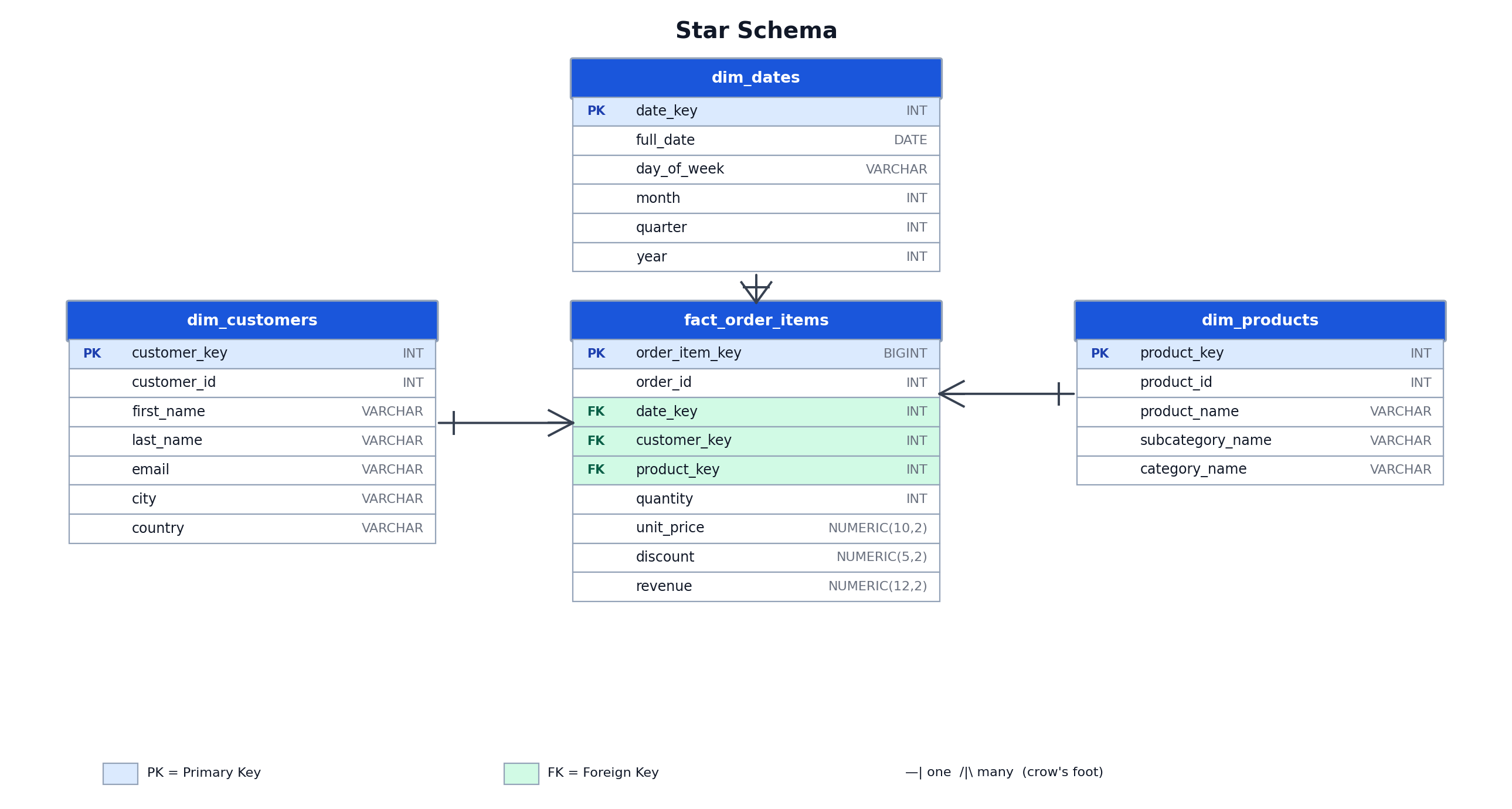
A prima schema organizes analytics information into a cardinal truth array surrounded by level magnitude tables. The shape, and the name, comes from the ER diagram: 1 array astatine the halfway pinch each magnitude tables pointing outward.
Core Components: Fact Tables and Flat Dimension Tables
A prima schema consists of a cardinal truth array surrounded by level magnitude tables. The truth array stores measurable events: bid statement items, page views, aliases sensor readings. Dimension tables shop the descriptive discourse for those events: merchandise attributes, customer details, and day hierarchies.
In a prima schema, magnitude tables are denormalized. All attributes for a concept, specified arsenic a product, are stored successful a azygous table, including some subcategory_name and category_name. A query aggregating gross by merchandise class joins the truth array to a azygous magnitude table. The sanction “star schema” describes the ocular style of the entity-relationship diagram, pinch the truth array astatine the halfway and magnitude tables radiating outward.
Star Schema DDL Example (Retail Sales Scenario)
CREATE TABLE dim_dates ( date_key INTEGER PRIMARY KEY, full_date DATE NOT NULL, day_of_week VARCHAR(10) NOT NULL, month INTEGER NOT NULL, 4th INTEGER NOT NULL, year INTEGER NOT NULL ); CREATE TABLE dim_customers ( customer_key INTEGER GENERATED BY DEFAULT AS IDENTITY PRIMARY KEY, customer_id INTEGER NOT NULL UNIQUE, first_name VARCHAR(100) NOT NULL, last_name VARCHAR(100) NOT NULL, email VARCHAR(255) NOT NULL, metropolis VARCHAR(100), state VARCHAR(100) ); CREATE TABLE dim_products ( product_key INTEGER GENERATED BY DEFAULT AS IDENTITY PRIMARY KEY, product_id INTEGER NOT NULL UNIQUE, product_name VARCHAR(255) NOT NULL, subcategory_name VARCHAR(100) NOT NULL, category_name VARCHAR(100) NOT NULL ); CREATE TABLE fact_order_items ( order_item_key BIGINT GENERATED BY DEFAULT AS IDENTITY PRIMARY KEY, order_id INTEGER NOT NULL, date_key INTEGER NOT NULL REFERENCES dim_dates(date_key), customer_key INTEGER NOT NULL REFERENCES dim_customers(customer_key), product_key INTEGER NOT NULL REFERENCES dim_products(product_key), amount INTEGER NOT NULL, unit_price NUMERIC(10,2) NOT NULL, discount NUMERIC(5,2) NOT NULL DEFAULT 0, gross NUMERIC(12,2) NOT NULL );The dim_products array stores subcategory_name and category_name arsenic nonstop columns. If a class sanction changes, each matching statement successful dim_products must beryllium updated individually.
When the Star Schema Is the Right Choice
The prima schema is the correct default for astir analytics workloads. If your BI instrumentality runs aggregation queries against a azygous magnitude astatine a time, the level building intends analysts tin constitute straightforward two-join queries without navigating a hierarchy. Tools that make SQL automatically, specified arsenic Metabase aliases Looker, thin to nutrient cleaner plans against prima schemas than against normalized ones.
The different information that favors a prima schema is ETL pipeline maturity. Denormalizing earlier load requires a tested, reliable pipeline. If yours is unchangeable and magnitude attributes successful your root strategy alteration rarely, you will not miss the update convenience that snowflake schemas provide. Start pinch a prima schema erstwhile simplicity matters much than storage.
What Is a Snowflake Schema successful PostgreSQL
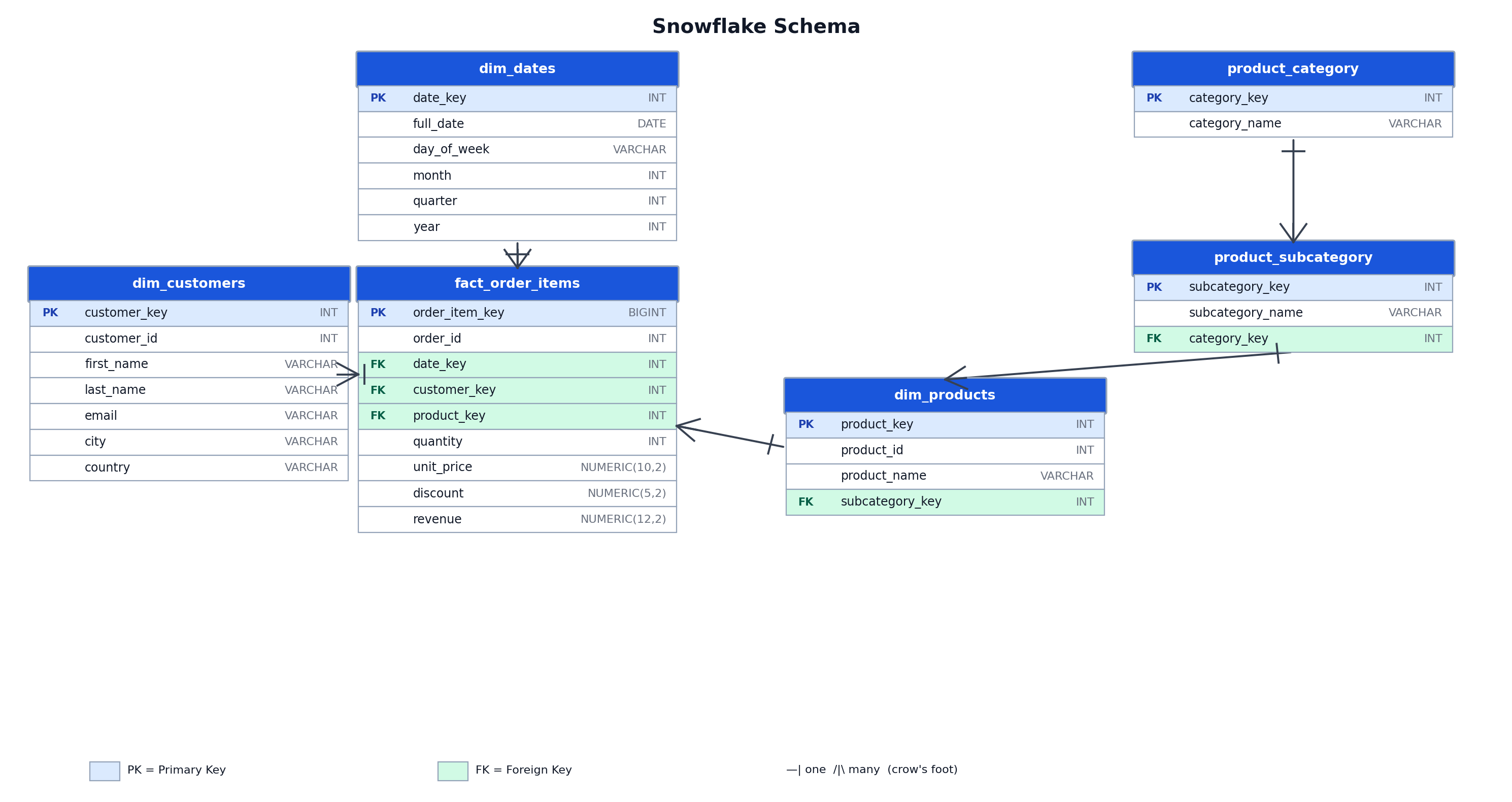
A snowflake schema starts pinch the aforesaid truth array but normalizes the magnitude tables into further lookup layers. The consequence is less redundant strings stored successful the database and much joins required per query.
How Normalization Extends the Dimension Tables
A snowflake schema applies normalization to magnitude tables. Instead of storing category_name straight successful dim_products, the merchandise magnitude references a product_subcategory table, which successful move references a product_category table. This removes the functional dependency betwixt subcategory_name and category_name from dim_products.
The trade-off is that queries requiring category-level aggregation must now subordinate 3 tables alternatively of one, traversing the level from fact_order_items done dim_products, product_subcategory, and product_category.
Snowflake Schema DDL Example (Same Retail Sales Scenario)
CREATE TABLE product_category ( category_key INTEGER GENERATED BY DEFAULT AS IDENTITY PRIMARY KEY, category_name VARCHAR(100) NOT NULL ); CREATE TABLE product_subcategory ( subcategory_key INTEGER GENERATED BY DEFAULT AS IDENTITY PRIMARY KEY, subcategory_name VARCHAR(100) NOT NULL, category_key INTEGER NOT NULL REFERENCES product_category(category_key) ); CREATE TABLE dim_dates ( date_key INTEGER PRIMARY KEY, full_date DATE NOT NULL, day_of_week VARCHAR(10) NOT NULL, month INTEGER NOT NULL, 4th INTEGER NOT NULL, year INTEGER NOT NULL ); CREATE TABLE dim_customers ( customer_key INTEGER GENERATED BY DEFAULT AS IDENTITY PRIMARY KEY, customer_id INTEGER NOT NULL UNIQUE, first_name VARCHAR(100) NOT NULL, last_name VARCHAR(100) NOT NULL, email VARCHAR(255) NOT NULL, metropolis VARCHAR(100), state VARCHAR(100) ); CREATE TABLE dim_products ( product_key INTEGER GENERATED BY DEFAULT AS IDENTITY PRIMARY KEY, product_id INTEGER NOT NULL UNIQUE, product_name VARCHAR(255) NOT NULL, subcategory_key INTEGER NOT NULL REFERENCES product_subcategory(subcategory_key) ); CREATE TABLE fact_order_items ( order_item_key BIGINT GENERATED BY DEFAULT AS IDENTITY PRIMARY KEY, order_id INTEGER NOT NULL, date_key INTEGER NOT NULL REFERENCES dim_dates(date_key), customer_key INTEGER NOT NULL REFERENCES dim_customers(customer_key), product_key INTEGER NOT NULL REFERENCES dim_products(product_key), amount INTEGER NOT NULL, unit_price NUMERIC(10,2) NOT NULL, discount NUMERIC(5,2) NOT NULL DEFAULT 0, gross NUMERIC(12,2) NOT NULL );When the Snowflake Schema Is the Right Choice
The snowflake schema earns its complexity erstwhile magnitude attributes alteration frequently. If your merchandise catalog is reorganized quarterly, updating 1 statement successful product_category is considerably cheaper than moving a batch UPDATE crossed 20,000 rows successful dim_products. At scale, that quality successful update costs is not theoretical.
Two different cases favour snowflake: shared dimensions and information governance requirements. If a product_category array is referenced by some a income truth array and an inventory truth table, normalizing it erstwhile prevents the 2 truth tables from diverging connected class names. For environments wherever referential integrity must beryllium enforced astatine the database level alternatively than successful the exertion layer, the overseas cardinal concatenation successful a snowflake schema does that activity automatically.
Star Schema vs Snowflake Schema: Direct Comparison
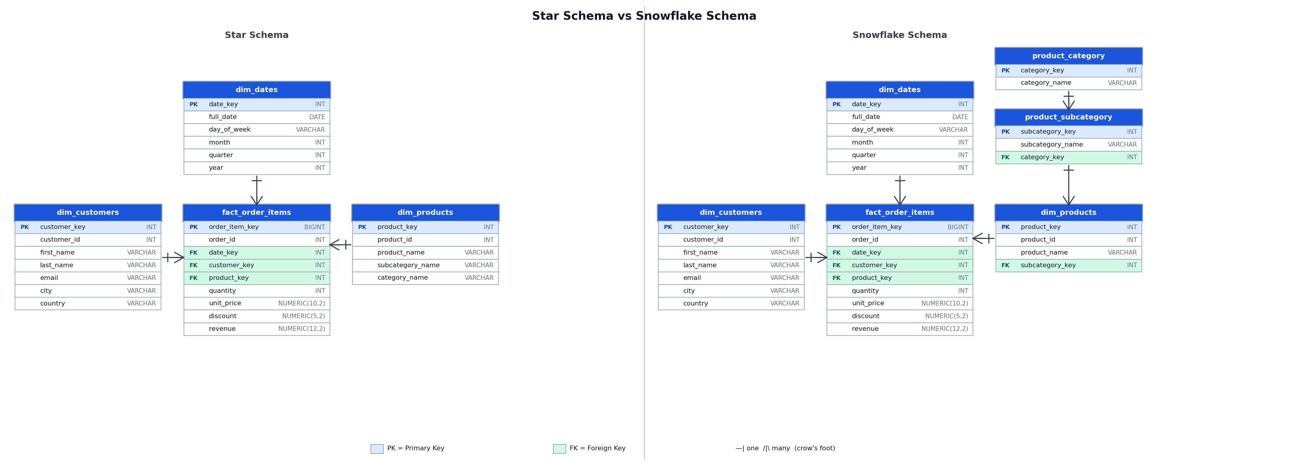
The applicable quality betwixt the 2 schemas is wherever you salary the cost: astatine query clip pinch snowflake, aliases astatine ETL load clip pinch star. The subsections beneath quantify that trade-off crossed the dimensions that matter astir successful production.
Query Complexity and Join Count
A prima schema query joining fact_order_items to dim_products and dim_dates requires 2 joins to nutrient gross by class and quarter. The balanced snowflake query requires 4 joins: fact_order_items to dim_products, dim_products to product_subcategory, product_subcategory to product_category, and fact_order_items to dim_dates.
PostgreSQL handles further hash joins efficiently erstwhile the smaller magnitude tables fresh successful memory. However, each further subordinate increases readying clip and the consequence of a suboptimal subordinate bid astatine precocious statement counts.
Storage Footprint and Data Redundancy
The retention mathematics is straightforward. Take dim_products astatine 20,000 rows: storing category_name and subcategory_name arsenic VARCHAR(100) columns connected each statement costs astir 4 MB for those attributes alone. Move them into product_category (5 rows) and product_subcategory (2,800 rows), and the aforesaid accusation fits successful nether 50 KB. That is simply a 98% simplification for 2 columns.
In practice, this seldom drives the schema determination astatine the magnitude array level. The truth array holds integer overseas keys successful some schemas, truthful the existent retention costs quality is successful the magnitude tables, not successful fact_order_items. Where the savings go meaningful is erstwhile magnitude tables person hundreds of thousands of rows pinch aggregate low-cardinality VARCHAR attributes, which is communal successful merchandise and surface science hierarchies.
ETL Pipeline and Data Loading Complexity
Loading a prima schema intends your ETL pipeline owns the denormalization step. Before inserting into dim_products, the pipeline has to subordinate the root merchandise array pinch class and subcategory lookups and flatten the consequence into a azygous row. When that pipeline is well-tested, this is simply a one-time cost. When it is not, you will spot class mismatches propagate silently into the magnitude table.
A snowflake schema shifts that burden. The normalized building maps much intimately to really root systems shop data, truthful magnitude loads require less transformations. The trade-off is that incremental loads request to support consistency crossed product_category, product_subcategory, and dim_products successful the correct order. Foreign cardinal constraints will drawback violations, but the coordination overhead is real.
Maintenance and Update Anomalies
A prima schema is susceptible to update anomalies. If a merchandise class sanction changes, each statement successful dim_products carrying that category_name must beryllium updated. With slow changing magnitude (SCD) Type 1 patterns, this tin require batch updates crossed ample magnitude tables.
A snowflake schema eliminates this for normalized attributes. Updating category_name successful product_category propagates implicitly to each products successful that class done the overseas cardinal relationship, astatine the costs of 1 statement update.
Comparison Table
| Star schema | Faster for astir aggregations; less joins | Lower; redundant property strings successful magnitude rows | Low; 1-2 joins for emblematic analytical queries | Higher; pipeline must denormalize earlier load | BI reporting, dashboard queries, unchangeable dimensions |
| Snowflake schema | Slower astatine scale; 2+ further joins per level level | Higher; normalized attributes stored once | Higher; 3-5 joins for hierarchy-traversing queries | Lower; pipeline mirrors root building much closely | Data governance environments, often updated dimensions, shared lookup tables |
Generating Test Data for Reproducible Benchmarks
The EXPLAIN ANALYZE outputs successful the adjacent conception were collected connected a production-representative dataset pinch a larger day scope than the generator below. Run these generate_series scripts against your analytics database to populate a functionally balanced dataset for schema validation and comparative benchmarking. Your scheme statement counts and timings will disagree proportionally; the comparative quality betwixt prima and snowflake query capacity is accordant crossed dataset sizes astatine this scale.
Populate dim_dates pinch 1 statement per almanac time from 2020 done 2025 (2,192 rows):
INSERT INTO dim_dates (date_key, full_date, day_of_week, month, quarter, year) SELECT TO_CHAR(d, 'YYYYMMDD')::INTEGER, d::DATE, TO_CHAR(d, 'FMDay'), EXTRACT(MONTH FROM d)::INTEGER, EXTRACT(QUARTER FROM d)::INTEGER, EXTRACT(YEAR FROM d)::INTEGER FROM generate_series('2020-01-01'::DATE, '2025-12-31'::DATE, '1 day') d;Populate dim_customers pinch 50,000 rows:
INSERT INTO dim_customers (customer_id, first_name, last_name, email, city, country) SELECT i, 'First' || i, 'Last' || i, 'customer' || one || '@example.com', (ARRAY['New York','San Francisco','Chicago','Austin','Seattle'])[1 + (i % 5)], 'US' FROM generate_series(1, 50000) i;Populate dim_products pinch 20,000 rows (star schema version):
INSERT INTO dim_products (product_id, product_name, subcategory_name, category_name) SELECT i, 'Product ' || i, (ARRAY['Laptops','Tablets','Phones','Monitors','Accessories', 'Chairs','Desks','Shelves','Lamps','Rugs', 'Jackets','Shirts','Pants','Shoes','Hats', 'Bats','Balls','Nets','Gloves','Helmets', 'Pans','Knives','Bowls','Plates','Cups'])[1 + (i % 25)], (ARRAY['Electronics','Furniture','Clothing','Sports','Kitchen'])[1 + (i % 5)] FROM generate_series(1, 20000) i;Populate fact_order_items pinch astir 2.7 cardinal rows:
INSERT INTO fact_order_items (order_id, date_key, product_key, customer_key, quantity, unit_price, discount, revenue) SELECT (random() * 500000 + 1)::INTEGER, TO_CHAR('2020-01-01'::DATE + floor(random() * 2192)::INTEGER, 'YYYYMMDD')::INTEGER, (random() * 19999 + 1)::INTEGER, (random() * 49999 + 1)::INTEGER, v.quantity, v.unit_price, v.discount, ROUND((v.quantity * v.unit_price) * (1 - v.discount), 2) AS revenue FROM generate_series(1, 2700000) CROSS JOIN LATERAL ( SELECT (random() * 10 + 1)::INTEGER AS quantity, (random() * 500 + 10)::NUMERIC(10,2) AS unit_price, 0::NUMERIC(5,2) AS discount ) v;Run ANALYZE aft loading to update planner statistic earlier benchmarking:
psql -d analytics -c "ANALYZE dim_dates, dim_customers, dim_products, fact_order_items;"The prima and snowflake versions of dim_products person incompatible file definitions, and fact_order_items references whichever type exists. Benchmark the 2 schemas successful abstracted databases, aliases driblet and recreate fact_order_items and dim_products pinch the snowflake DDL earlier moving the artifact below. Running some schema definitions successful the aforesaid database without recreating these tables will neglect because the snowflake INSERT omits the subcategory_name and category_name columns that the prima dim_products requires.
For the snowflake schema benchmark, populate the normalized magnitude tables utilizing the aforesaid 5-category, 2,800-subcategory building (560 subcategories per category):
INSERT INTO product_category (category_name) VALUES ('Electronics'), ('Furniture'), ('Clothing'), ('Sports'), ('Kitchen'); INSERT INTO product_subcategory (subcategory_name, category_key) SELECT pc.category_name || ' Sub ' || s, pc.category_key FROM product_category pc CROSS JOIN generate_series(1, 560) s; INSERT INTO dim_products (product_id, product_name, subcategory_key) SELECT i, 'Product ' || i, (SELECT subcategory_key FROM product_subcategory ORDER BY subcategory_key OFFSET (i % 2800) LIMIT 1)Run ANALYZE connected the snowflake magnitude tables aft loading:
psql -d analytics -c "ANALYZE product_category, product_subcategory;"Query Performance connected PostgreSQL: What the Numbers Show
Schema prime affects query plans successful 2 measurable ways: subordinate count and hash array representation usage. The EXPLAIN ANALYZE outputs beneath show some connected the aforesaid 2.7 million-row truth array truthful the costs quality is straight comparable.
EXPLAIN ANALYZE Output for a Star Schema Aggregation Query
The EXPLAIN ANALYZE outputs beneath were generated connected a DigitalOcean Managed PostgreSQL 15 cluster (4 vCPU, 8 GB RAM) pinch work_mem group to 64 MB. Row counts and timing values will disagree connected your cluster based connected array statistics, representation configuration, and PostgreSQL version. The comparative quality betwixt the 2 schema types is typical of a denormalized vs. normalized magnitude level astatine this statement count.
This query aggregates gross by merchandise class and 4th connected a fact_order_items array pinch astir 2.7 cardinal rows.
EXPLAIN ANALYZE SELECT dp.category_name, dd.year, dd.quarter, SUM(foi.revenue) AS total_revenue, COUNT(DISTINCT foi.order_id) AS order_count FROM fact_order_items foi JOIN dim_products dp ON foi.product_key = dp.product_key JOIN dim_dates dd ON foi.date_key = dd.date_key WHERE dd.year = 2023 AND dp.category_name = 'Electronics' GROUP BY dp.category_name, dd.year, dd.quarter ORDER BY dd.quarter; HashAggregate (cost=84321.50..84325.80 rows=16 width=48) (actual time=412.344..412.591 rows=4 loops=1) Group Key: dp.category_name, dd.year, dd.quarter -> Hash Join (cost=1628.90..82944.30 rows=89918 width=32) (actual time=20.344..387.801 rows=89918 loops=1) Hash Cond: (foi.date_key = dd.date_key) -> Hash Join (cost=1592.00..71308.20 rows=540000 width=28) (actual time=18.211..298.112 rows=540000 loops=1) Hash Cond: (foi.product_key = dp.product_key) -> Seq Scan connected fact_order_items foi (cost=0.00..52130.00 rows=2700000 width=24) (actual time=0.021..142.430 rows=2700000 loops=1) -> Hash (cost=1592.00..1592.00 rows=4000 width=20) (actual time=10.411..10.412 rows=4000 loops=1) Buckets: 4096 Batches: 1 Memory Usage: 309kB -> Seq Scan connected dim_products dp (cost=0.00..1592.00 rows=4000 width=20) (actual time=0.011..6.322 rows=4000 loops=1) Filter: (category_name = 'Electronics') Rows Removed by Filter: 16000 -> Hash (cost=36.90..36.90 rows=365 width=12) (actual time=2.511..2.512 rows=365 loops=1) Buckets: 1024 Batches: 1 Memory Usage: 26kB -> Seq Scan connected dim_dates dd (cost=0.00..36.90 rows=365 width=12) (actual time=0.009..1.234 rows=365 loops=1) Filter: (year = 2023) Rows Removed by Filter: 1827 Planning Time: 2.341 ms Execution Time: 413.019 msPostgreSQL chose hash joins for some magnitude lookups. The select connected category_name runs against the in-memory hash of dim_products, truthful each 2.7 cardinal truth rows are publication precisely once.
EXPLAIN ANALYZE Output for the Equivalent Snowflake Schema Query
EXPLAIN ANALYZE SELECT pc.category_name, dd.year, dd.quarter, SUM(foi.revenue) AS total_revenue, COUNT(DISTINCT foi.order_id) AS order_count FROM fact_order_items foi JOIN dim_products dp ON foi.product_key = dp.product_key JOIN product_subcategory ps ON dp.subcategory_key = ps.subcategory_key JOIN product_category microcomputer ON ps.category_key = pc.category_key JOIN dim_dates dd ON foi.date_key = dd.date_key WHERE dd.year = 2023 AND pc.category_name = 'Electronics' GROUP BY pc.category_name, dd.year, dd.quarter ORDER BY dd.quarter; HashAggregate (cost=99812.40..99816.70 rows=16 width=48) (actual time=498.712..498.981 rows=4 loops=1) Group Key: pc.category_name, dd.year, dd.quarter -> Hash Join (cost=505.95..98180.20 rows=89918 width=32) (actual time=22.341..471.229 rows=89918 loops=1) Hash Cond: (foi.date_key = dd.date_key) -> Hash Join (cost=469.05..95100.40 rows=540000 width=28) (actual time=20.114..421.902 rows=540000 loops=1) Hash Cond: (ps.category_key = pc.category_key) -> Hash Join (cost=468.00..88444.30 rows=2700000 width=32) (actual time=12.123..360.112 rows=2700000 loops=1) Hash Cond: (dp.subcategory_key = ps.subcategory_key) -> Hash Join (cost=412.00..80305.60 rows=2700000 width=28) (actual time=8.344..288.112 rows=2700000 loops=1) Hash Cond: (foi.product_key = dp.product_key) -> Seq Scan connected fact_order_items foi (cost=0.00..52130.00 rows=2700000 width=24) (actual time=0.021..142.430 rows=2700000 loops=1) -> Hash (cost=412.00..412.00 rows=20000 width=8) (actual time=8.111..8.112 rows=20000 loops=1) Buckets: 32768 Batches: 1 Memory Usage: 940kB -> Seq Scan connected dim_products dp (cost=0.00..412.00 rows=20000 width=8) (actual time=0.011..3.902 rows=20000 loops=1) -> Hash (cost=56.00..56.00 rows=2800 width=8) (actual time=3.211..3.212 rows=2800 loops=1) Buckets: 4096 Batches: 1 Memory Usage: 142kB -> Seq Scan connected product_subcategory ps (cost=0.00..56.00 rows=2800 width=8) (actual time=0.009..1.512 rows=2800 loops=1) -> Hash (cost=1.05..1.05 rows=1 width=12) (actual time=0.018..0.019 rows=1 loops=1) Buckets: 1024 Batches: 1 Memory Usage: 9kB -> Seq Scan connected product_category pc (cost=0.00..1.05 rows=1 width=12) (actual time=0.007..0.011 rows=1 loops=1) Filter: (category_name = 'Electronics') Rows Removed by Filter: 4 -> Hash (cost=36.90..36.90 rows=365 width=12) (actual time=2.511..2.512 rows=365 loops=1) Buckets: 1024 Batches: 1 Memory Usage: 26kB -> Seq Scan connected dim_dates dd (cost=0.00..36.90 rows=365 width=12) (actual time=0.009..1.234 rows=365 loops=1) Filter: (year = 2023) Rows Removed by Filter: 1827 Planning Time: 3.812 ms Execution Time: 499.621 msThe snowflake query ran successful 499 sclerosis against 413 sclerosis for the prima schema query, a 21% quality connected the aforesaid 2.7 cardinal truth rows. In the scheme shown, PostgreSQL joins dim_products to the afloat product_subcategory group (2,800 rows) earlier applying the pc.category_name = 'Electronics' select astatine the product_category join. Depending connected array statistic and configuration, the planner whitethorn alternatively take a subordinate bid that applies the class regularisation earlier.
Index Strategies for Fact Tables connected Managed PostgreSQL
Three scale strategies reside the astir communal analytics bottlenecks connected fact_order_items.
BRIN (Block Range Index) is businesslike for columns wherever values are correlated pinch beingness retention order, which is emblematic for append-only truth tables loaded successful day order:
CREATE INDEX idx_fact_order_items_date_brin ON fact_order_items USING BRIN (date_key);A partial scale limits scope to caller periods, reducing scale size and attraction overhead erstwhile reports attraction connected existent data:
CREATE INDEX idx_fact_order_items_recent ON fact_order_items (date_key, product_key) WHERE date_key >= 20240101;A covering scale allows the planner to fulfill a communal aggregation query from the scale without a heap scan:
CREATE INDEX idx_fact_order_items_covering ON fact_order_items (date_key, product_key) INCLUDE (revenue, order_id);Run ANALYZE fact_order_items; aft bulk loads to refresh planner statistics. Stale statistic origin the planner to take suboptimal subordinate orders, which is the astir communal origin of unexpected capacity regression successful analytics schemas. Also tally VACUUM fact_order_items; aft bulk loads truthful the visibility representation is existent and the planner tin usage index-only scans against the covering index. Without a caller VACUUM, heap fetches bypass the scale moreover erstwhile the covering scale contains each required columns.
Setting Up Your Analytics Schema connected DigitalOcean Managed PostgreSQL
The steps beneath screen cluster provisioning, analytics-specific parameter configuration, schema application, and relationship pooling for some schema types connected DigitalOcean Managed PostgreSQL.
Provisioning a Managed PostgreSQL Cluster for Analytics Workloads
Navigate to the DigitalOcean Managed PostgreSQL merchandise page and prime a scheme pinch astatine slightest 4 GB RAM. Analytics queries involving multi-join snowflake schemas use from higher representation configurations because PostgreSQL allocates work_mem per hash cognition during subordinate execution. For clusters pinch read-heavy analytics workloads, provisioning a publication replica and routing study queries to the replica isolates analytics load from transactional operations connected the primary.
Configuring work_mem and enable_hashjoin for Multi-Join Queries
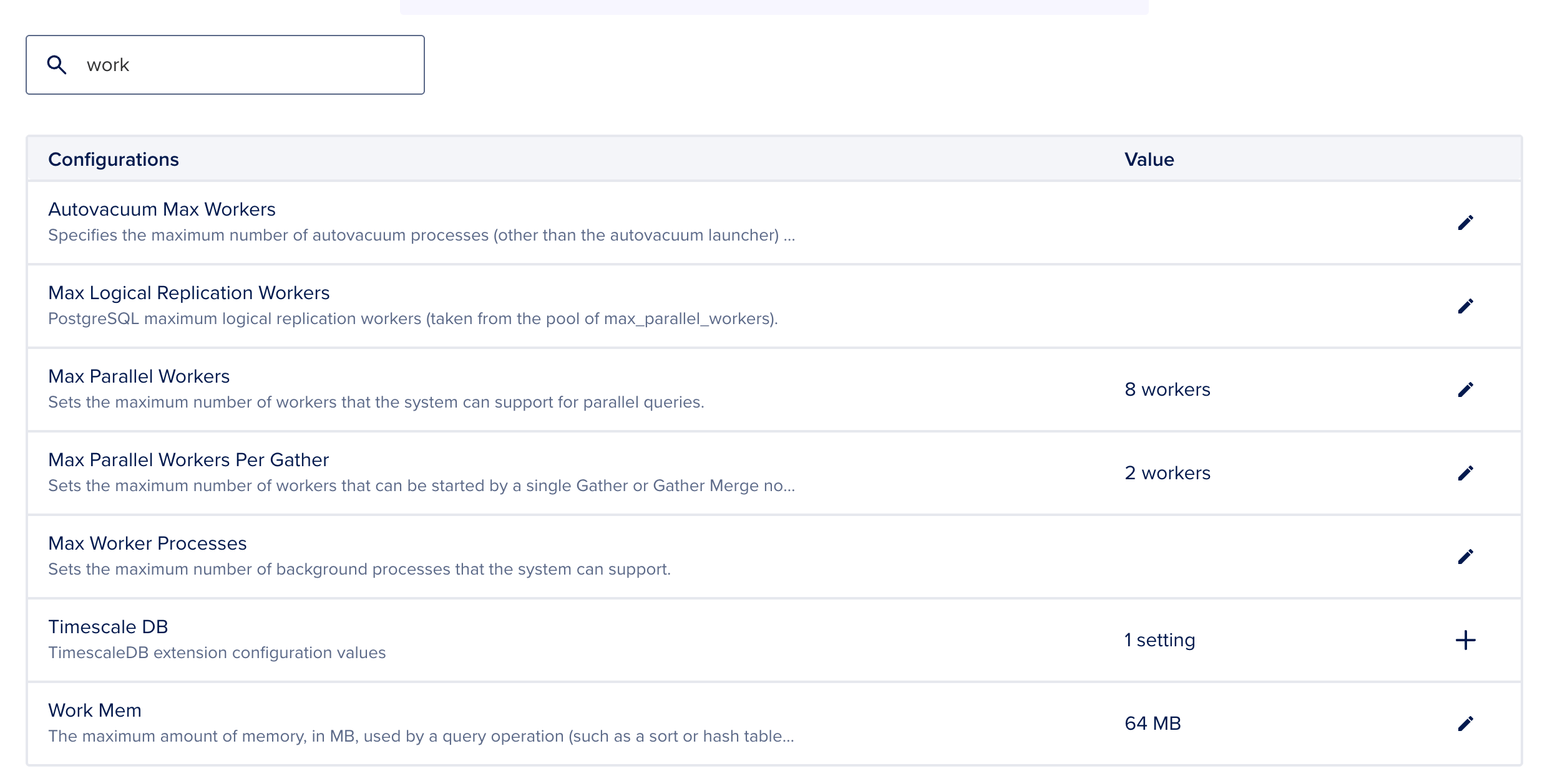
On DigitalOcean Managed PostgreSQL, configure analytics parameters done the cluster settings sheet nether Advanced Configurations. The parameters astir applicable to multi-join query capacity are work_mem, max_parallel_workers_per_gather, and enable_hashjoin.
Recommended starting values for an analytics-focused cluster:
| work_mem | 256MB | Allocates representation per hash operation; reduces disk spill for snowflake multi-join queries |
| max_parallel_workers_per_gather | 4 | Enables parallel sequential scans connected ample truth tables |
| enable_hashjoin | on | Keeps hash subordinate plans enabled; should stay connected for analytics workloads |
ALTER SYSTEM is not disposable connected DigitalOcean Managed PostgreSQL. Configure these parameters done the power sheet nether Settings > Advanced Configurations aliases via the DigitalOcean API. Setting work_mem excessively precocious connected shared clusters tin origin out-of-memory conditions nether concurrent load. Test pinch session-level overrides first: SET work_mem = '256MB';
For a session-level override earlier moving a circumstantial analytics query:
SET work_mem = '256MB';This applies only to the existent relationship and is compatible pinch PgBouncer successful convention pooling mode.
Applying the Star aliases Snowflake Schema pinch psql aliases pgAdmin
After connecting to your managed cluster, use the DDL from the erstwhile sections utilizing psql. If you request to group up a PostgreSQL client, spot How To Install and Use PostgreSQL connected Ubuntu 22.04 for relationship instructions.
psql "postgresql://doadmin:<password>@<cluster-host>:25060/analytics?sslmode=verify-full&sslrootcert=/path/to/ca-certificate.crt" \ -f star_schema.sqlFor pgAdmin, unfastened the Query Tool, paste each DDL block, and execute. Create a dedicated analytics database earlier moving schema DDL to support analytics tables isolated from exertion databases connected the aforesaid cluster.
Table Partitioning and Schema Interaction
Range partitioning connected date_key is compatible pinch some prima and snowflake schemas and is the modular attack for truth tables that turn beyond 50 cardinal rows. Partition the truth array by twelvemonth aliases 4th utilizing PARTITION BY RANGE:
CREATE TABLE fact_order_items ( order_item_key BIGINT GENERATED BY DEFAULT AS IDENTITY, order_id INTEGER NOT NULL, date_key INTEGER NOT NULL, product_key INTEGER NOT NULL, customer_key INTEGER NOT NULL, amount INTEGER NOT NULL, unit_price NUMERIC(10,2) NOT NULL, discount NUMERIC(5,2) NOT NULL DEFAULT 0, gross NUMERIC(12,2) NOT NULL ) PARTITION BY RANGE (date_key); CREATE TABLE fact_order_items_2024 PARTITION OF fact_order_items FOR VALUES FROM (20240101) TO (20250101); CREATE TABLE fact_order_items_2025 PARTITION OF fact_order_items FOR VALUES FROM (20250101) TO (20260101);A BRIN scale connected date_key wrong each partition reduces scale size further because BRIN indexes are built per partition and each partition has a narrower worth scope than the afloat table. Both prima and snowflake schemas use arsenic from partitioning because the truth array building is identical successful some patterns. The magnitude tables are not partitioned.
DigitalOcean Managed PostgreSQL supports declarative partitioning without superuser access. Create partition tables utilizing psql aliases pgAdmin connected to the cluster arsenic the doadmin user.
Connection Pooling Considerations pinch PgBouncer
DigitalOcean Managed PostgreSQL includes a built-in PgBouncer relationship pooler. For analytics workloads, usage convention pooling mode alternatively than transaction pooling mode.
Transaction pooling returns connections to the excavation aft each statement, which is incompatible pinch session-level SET work_mem overrides and pinch prepared connection caching utilized by immoderate BI tools. Create a dedicated relationship excavation for analytics connections successful the Managed Database power sheet nether Connection Pools, and configure it pinch convention mode and a excavation size due for your concurrent analytics query load.
Normalization vs Denormalization: The Core Trade-off
Neither shape is unconditionally better. The correct prime depends connected really often magnitude attributes change, really galore truth tables stock those dimensions, and what your ETL pipeline tin reliably nutrient astatine load time.
When Denormalization Serves Analytics Workloads
Denormalization reduces the number of tables a query must touch to nutrient a result. For read-heavy OLAP workloads wherever information is loaded successful nightly aliases hourly batches and seldom updated successful place, storing redundant property values successful level magnitude tables is usually an acceptable costs for the query simplicity it provides.
A level dim_products array besides benefits BI devices pinch constricted query optimization. Some spreadsheet-based connectors and embedded analytics libraries make single-join aggregation queries and cannot traverse multi-table hierarchies without manual configuration.
When Normalization Reduces Long-Term Storage and Update Costs
Normalization provides the astir use erstwhile magnitude attributes person debased cardinality and precocious repetition. In a larger deployment, if dim_products has 100,000 rows and category_name takes 1 of 5 imaginable values, storing the afloat drawstring 100,000 times is wasteful compared to 5 rows successful product_category and an integer overseas cardinal successful dim_products.
The update costs advantage is important pinch SCD Type 1 patterns, wherever property changes overwrite humanities values. A azygous UPDATE to 1 statement successful product_category is cheaper and little error-prone than a batch UPDATE crossed 10,000 rows successful dim_products.
Hybrid Approaches: Partially Normalized Dimensions
A hybrid schema normalizes high-cardinality, often updated magnitude attributes while keeping low-cardinality, unchangeable attributes flat. You mightiness normalize product_category and product_subcategory into abstracted tables because they alteration occasionally and are shared crossed aggregate truth tables, while keeping customer reside attributes level successful dim_customers because addresses are unsocial per customer and seldom grouped successful analytical queries.
This attack is communal successful accumulation PostgreSQL information warehouses wherever different dimensions person different operational characteristics and update frequencies.
Choosing Between Star and Snowflake Schema: A Decision Framework
Use the checklist beneath erstwhile starting a caller analytics task aliases evaluating whether an existing schema is causing much operational clash than it solves.
The determination norm successful 1 sentence: If your astir predominant BI queries traverse a magnitude level connected a truth array supra 50 cardinal rows, a prima schema will beryllium measurably faster than the balanced snowflake schema connected the aforesaid managed PostgreSQL cluster. Below 10 cardinal rows, the quality is dominated by scale value and work_mem configuration, not schema choice.
Decision Criteria Checklist
- Dimension update frequency: if magnitude attributes alteration much than monthly, favour snowflake to trim update anomalies.
- Fact array statement count: beneath 10 cardinal rows, the query capacity quality is usually negligible pinch due indexing; supra 50 cardinal rows, benchmark some schemas pinch typical queries earlier committing.
- BI instrumentality SQL generation: if your instrumentality generates SQL automatically, verify it produces businesslike multi-join queries; prima schemas are safer for devices pinch constricted query optimization.
- Shared dimensions: if the aforesaid lookup information appears successful aggregate truth tables, normalizing it into shared magnitude tables prevents property divergence.
- ETL pipeline maturity: denormalization requires a reliable, tested ETL process; if your pipeline is early-stage, commencement pinch snowflake and denormalize later erstwhile the pipeline is stable.
- Team SQL proficiency: snowflake schemas require much analyzable query authoring; if your analysts are little knowledgeable pinch multi-table joins, prima schemas trim friction.
Signals That Indicate You Should Migrate from One Schema to the Other
Migrate from prima to snowflake erstwhile magnitude array updates are becoming costly owed to high-cardinality redundant attributes, aliases erstwhile aggregate truth tables request to stock magnitude information and synchronization is failing.
Migrate from snowflake to prima erstwhile EXPLAIN ANALYZE output consistently shows subordinate overhead arsenic the bottleneck connected your astir predominant BI reports, and erstwhile your ETL pipeline tin reliably denormalize dimensions earlier loading.
Migrating Between Schemas Without Downtime
Use the view-swap shape to migrate from a snowflake schema to a prima schema without taking the database offline aliases blocking reads. The afloat process pinch SQL is covered successful the FAQ reply for migration, but the operational series is:
- Create a denormalized position of the snowflake magnitude hierarchy.
- Validate the position returns correct statement counts and file values against your existing queries.
- Create the caller beingness prima schema array utilizing the aforesaid file names and types arsenic the view.
- Backfill the array from the position wrong a transaction.
- In a azygous transaction, rename the original tables and switch successful the caller prima schema table.
- Drop the normalized lookup tables aft confirming each queries way correctly to the caller table.
The position acts arsenic a statement betwixt the aged schema and the caller one: queries proceed moving against the position during the migration window, and the beingness switch is instant astatine the DDL level.
Frequently Asked Questions
Q: Is prima schema ever faster than snowflake schema successful PostgreSQL?
Not always. The capacity quality depends connected subordinate count, array sizes, work_mem configuration, and scale coverage. A prima schema requires less hash subordinate operations than the balanced snowflake query for the aforesaid truth table, truthful it tends to beryllium faster for hierarchy-traversing aggregations. At debased statement counts the quality is often negligible. The PostgreSQL query planner optimizes hash subordinate sequences based connected statistic collected by ANALYZE; old statistic origin much capacity degradation than the schema prime itself, truthful moving ANALYZE aft bulk loads has much effect connected query latency than schema action astatine mini scale.
Q: Does PostgreSQL grip snowflake schema joins efficiently astatine scale?
At precocious statement counts pinch insufficient work_mem, the planner starts spilling intermediate hash tables to disk. The much joins your snowflake query requires, the much apt this is to happen, and the larger the capacity spread comparative to an balanced prima schema query. Increasing work_mem to 128-256 MB connected DigitalOcean Managed PostgreSQL reduces disk spill and narrows the gap; the nonstop betterment depends connected your truth array size, subordinate count, and concurrency level. Run ANALYZE aft loading caller magnitude data. Stale statistic origin the planner to prime the incorrect subordinate order, and that has much effect connected snowflake queries than connected prima schema queries because location are much joins to get wrong.
Q: Can I usage some prima and snowflake patterns successful the aforesaid PostgreSQL database?
Yes. Different taxable areas successful the aforesaid database tin usage different schema patterns. A income taxable area mightiness usage a prima schema pinch a level dim_products table, while an inventory taxable area uses a snowflake schema pinch normalized product_subcategory and product_category tables. The product_category array successful the snowflake schema tin service arsenic a shared magnitude by adding a overseas cardinal from the prima schema’s dim_products to it, combining some patterns successful a hybrid design. This is simply a applicable attack erstwhile different taxable areas person different query entree patterns and update frequencies.
Q: How does retention costs disagree betwixt prima and snowflake schemas connected DigitalOcean Managed PostgreSQL?
For a actual estimate: dim_products pinch 20,000 rows storing 2 VARCHAR(100) attributes uses astir 4 MB for those columns. Normalizing those attributes into product_category (5 rows) and product_subcategory (2,800 rows) reduces that to nether 50 KB. The truth array stores integer overseas keys successful some schemas, truthful the retention quality is successful the magnitude tables, not successful fact_order_items. On managed PostgreSQL wherever retention is billed by the gigabyte, snowflaking magnitude tables typically saves little than 1% of full retention for a schema pinch a decently designed truth table. Storage savings are much important erstwhile magnitude tables person precocious statement counts (above 500,000) pinch aggregate low-cardinality attributes.
Q: What PostgreSQL scale types activity champion for truth tables successful a prima schema?
BRIN indexes activity good for date_key columns successful append-only truth tables wherever statement values are correlated pinch insertion order. A BRIN scale connected date_key is orders of magnitude smaller than a B-tree scale connected the aforesaid file and has little attraction overhead during bulk inserts. For overseas cardinal columns specified arsenic product_key and customer_key, B-tree indexes are useful erstwhile queries select selectively connected those keys and erstwhile the planner chooses nested-loop aliases merge joins. Covering indexes utilizing the INCLUDE clause are effective for queries that aggregate gross grouped by date_key and product_key: the planner tin fulfill the query from the scale without accessing the heap, which reduces I/O importantly connected ample truth tables.
Q: How do I migrate from a snowflake schema to a prima schema successful PostgreSQL without downtime?
Follow these steps to migrate without downtime:
- Create a denormalized position of the snowflake dimension.
- Validate the position against your existing queries.
- Create the caller beingness prima schema table.
- Backfill the array from the view.
- In a azygous transaction, rename the aged array and switch successful the caller one.
- Drop the normalized tables aft verifying each queries way correctly.
For measurement 1, create a denormalized position of the snowflake dimension:
CREATE VIEW v_dim_products_flat AS SELECT dp.product_key, dp.product_id, dp.product_name, ps.subcategory_name, pc.category_name FROM dim_products dp JOIN product_subcategory ps ON dp.subcategory_key = ps.subcategory_key JOIN product_category microcomputer ON ps.category_key = pc.category_key;For measurement 3, create the beingness prima schema table:
CREATE TABLE dim_products_star ( product_key INTEGER GENERATED BY DEFAULT AS IDENTITY PRIMARY KEY, product_id INTEGER NOT NULL UNIQUE, product_name VARCHAR(255) NOT NULL, subcategory_name VARCHAR(100) NOT NULL, category_name VARCHAR(100) NOT NULL );For measurement 4, backfill from the view:
INSERT INTO dim_products_star SELECT product_key, product_id, product_name, subcategory_name, category_name FROM v_dim_products_flat;After backfilling, validate statement counts lucifer betwixt v_dim_products_flat and dim_products_star earlier proceeding to the switch successful measurement 5.
Q: Does DigitalOcean Managed PostgreSQL support the configuration changes needed for analytics workloads?
Yes. The pursuing parameters are configurable done the DigitalOcean power sheet nether Settings > Advanced Configurations, aliases via the DigitalOcean API:
- work_mem: controls representation per benignant aliases hash operation; expanding this reduces disk spill for multi-join snowflake queries.
- max_parallel_workers_per_gather: controls parallel workers utilized for sequential scans and aggregations; expanding from the default of 2 to 4 aliases 8 connected larger clusters reduces scan clip connected ample truth tables.
- enable_hashjoin: group to connected by default; controls whether the planner considers hash subordinate plans.
Parameters not configurable connected managed PostgreSQL see shared_buffers (set automatically based connected cluster size) and superuser-only parameters. max_connections is configurable wrong scheme limits.
Q: What is the quality betwixt a snowflake schema and 3rd normal shape (3NF) successful a information warehouse?
Third normal shape (3NF) is simply a normalization modular designed for transactional databases to destruct update anomalies successful operational systems. A snowflake schema borrows the aforesaid structural rule but applies it selectively to magnitude tables successful an analytical context. In a strict 3NF transactional schema, each non-key property must dangle only connected the superior cardinal of its table. In a snowflake schema, the truth array is intentionally not successful 3NF: it stores additive measures for illustration gross and amount alongside aggregate overseas keys, because those measures dangle connected the operation of keys, not a azygous key. The magnitude hierarchies are normalized, but the wide schema is not successful 3NF. The extremity of snowflaking is not afloat normalization but controlled normalization of circumstantial property hierarchies that person update anomaly risks aliases retention overhead worthy addressing.
Conclusion
Star and snowflake schemas are not competing standards truthful overmuch arsenic 2 points connected a trade-off curve betwixt query simplicity and information exemplary integrity. This tutorial walked done some patterns successful full, from DDL to EXPLAIN ANALYZE output connected 2.7 cardinal truth rows, covering really the further hash subordinate operations successful a snowflake query impact query scheme shape, really to reside that pinch scale and configuration choices, and what conditions successful your ain workload should push you toward 1 schema aliases the other.
With these DDL examples and the determination model successful the last section, you tin proviso a DigitalOcean Managed PostgreSQL cluster, use the schema that fits your workload, and configure work_mem, relationship pooling, and indexes for analytics query performance. The comparison array and checklist supply a repeatable process for evaluating schema choices arsenic information measurement and squad requirements evolve.
As a actual adjacent step, tally the EXPLAIN ANALYZE queries from this tutorial connected some schemas, past adhd 2 much typical reports: a single-dimension aggregation and a filtered multi-dimension GROUP BY pinch a day scope predicate. Compare readying clip and execution clip for each pair. The results will corroborate whether your workload sits successful the authorities wherever schema prime drives capacity aliases wherever scale value and work_mem configuration are the ascendant factors. To adhd a earthy connection query furniture connected apical of your analytics schema, DigitalOcean AI Platform supports text-to-SQL procreation against a connected PostgreSQL schema, letting analysts query some schema types without penning SQL directly.
 This activity is licensed nether a Creative Commons Attribution-NonCommercial- ShareAlike 4.0 International License.


")


.png "Build A Medical Report Analyzer On Dedicated Inference With Python")


![Convince Your Boss To Send You To Mozcon 2026 [plus Bonus Letter Template]](https://moz.com/images/blog/Blog-OG-images/Convince-Your-Boss-to-Send-You-to-MozCon-OG-Image-3.png?w=1200&h=630&q=82&auto=format&fit=clip&dm=1751528541&s=53746c4b2d83c4c442cb78b9ca076247 "Convince Your Boss To Send You To Mozcon 2026 [plus Bonus Letter Template]")
") English (US) ·
English (US) · ") Indonesian (ID) ·
Indonesian (ID) ·