The Art of Dithering and Retro Shading for the Web

I spent the former few months construction my personal website from the dirt up, eventually taking the period to merge several 3D activity to showcase my shader and WebGL skills. Throughout this work, I got to really comprehend the crucial function that post-processing plays in making a environment really look good, which brought several resolutions to long-term frustrations I had alongside my former React Three Fiber and shader projects anywhere my imagination wouldn't materialize despite of the amount of activity and attention I was putting into them.

Taking the period to build, combine, and test alongside tradition post-processing effects gave me an additional imaginative outlet, and among the many types I got to iterate on, I continually had a particular affection for the multiple "retro" effects I came up with. With subtle particulars specified as dithering, color quantization, or pixelization/CRT RGB cells, they bring a pleasant difference between the contemporary web landscape and a long-gone era of innovation we 90s/early 2000s kids are sometime longing for.

Given the period I invested dissecting all aspect of these effects, I wanted to dive profound alongside you into the concepts powering them and the shader techniques I learned alongside the way. In this article, I anticipation to convince you of the power of post-processing effects and that nothing strikes an elegant retro vibe applied to a website 👌✨. We'll additionally appearance into examples of dithering and pixel art from extremely gifted folks who use the identical processes that I'll be introducing afterward on, as fine as several of my own creations that I built during learning concerning all this.

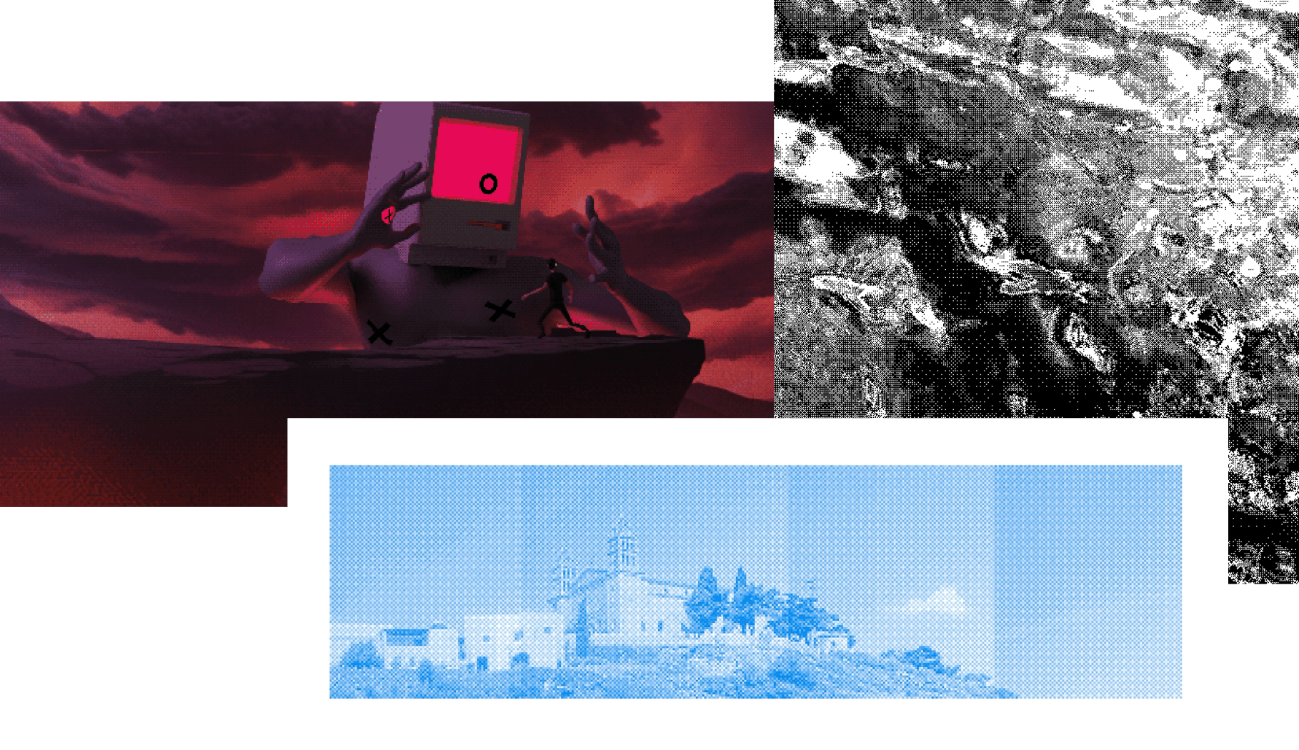
Dithering originated as an first graphics method to trick the viewer's brain into seeing additional color or smoothness in gradients/shadows that the machines rear in the day could output by intentionally introducing noise on top of an depiction or a render. Color palettes were extremely constricted rear then, thus relying on techniques akin these was critical for equivalent designers to acknowledge their vision. This gave, as a result, a distinctive appearance and awareness to games and media from that particular instant in period anywhere computers became ubiquitous, but advanced explanatory capabilities were not yet there.

Today, dithering is additional an imaginative choice than a workaround. Many artists or equivalent designers use this method as a imaginative outlet to provision their activity a distinctive retro vibe, calling out to that first gaming era, or activity inside the realms of self-imposed limits in colors. Some awesome examples of specified use of dithering include:

• Basement Studio's Basement Chronicle game: a well-executed point-and-click equivalent that reminds me a lot of my own first gaming experience.

• @loackme's art, which I'm an complete fan of.

• @aweusmeuh's use of the first Game Boy camera for experimental photography which features a sublime dithering effect.

The second is how we volition method dithering in this blog post: to provision our React Three Fiber/Three.js projects a distinctive style! In this archetypal part, we'll examine how the dithering method works, execute it as a shader, and build a archetypal repeat of a tradition dithering post-processing consequence that we can use on top of any 3D scene.

A archetypal continue at dithering in React Three Fiber

For this project, we'll create a custom post-processing effect. As we did for the Moebius stylized shader, relying on post-processing volition authorize us to use a shader to an already rendered environment and alter its manner akin adding an "image filter" to a photo.

To create a tradition effect, we will:

1. Declare a category that extends from Effect

2. Define our part shader and call it from the genitor constructor using the excellent keyword.

3. Define the set of uniforms we volition need for our effect.

4. Call the wrapEffect function from @react-three/post-processing alongside our consequence category as an argument. This volition authorize us to use our consequence as a JSX component inside EffectComposer.

1
import { OrbitControls, OrthographicCamera, useFBO } from '@react-three/drei';
2
import { Canvas } from '@react-three/fiber';
3
import { wrapEffect, EffectComposer } from '@react-three/postprocessing';
4
import { Effect } from 'postprocessing';
5
import { Suspense, useRef, useState } from 'react';
6
import { v4 as uuidv4 } from 'uuid';
8
import fragmentShader from './fragmentShader.glsl';
10
class RetroEffectImpl extends Effect {
12
 super('RetroEffect', fragmentShader, {
13
 uniforms: new Map([]),
18
const RetroEffect = wrapEffect(RetroEffectImpl);
21
 const mesh = useRef();
25
 <mesh receiveShadow castShadow>
26
 <torusKnotGeometry args={[1, 0.25, 128, 100]} />
27
 <meshStandardMaterial color="cyan" />

As a archetypal stage to construction our effect, we'll commencement alongside a uncomplicated luminance-based pale noise dithering. The idea rearward this is to:

• Look at the luminance of all pixel.

• Compare it to a random figure (hence the "white noise" in the name).

• Output a pale or dreary pixel according to whether the luminance falls complete or below stated random number.

2
 return fract(sin(dot(c.xy, vec2(12.9898, 78.233))) * 43758.5453);
5
vec3 whiteNoiseDither(vec2 uv, float lum) {
6
 vec3 color = vec3(0.0);
8
 if (lum < random(uv)) {
17
void mainImage(const in vec4 inputColor, const in vec2 uv, out vec4 outputColor) {
18
 vec4 color = texture2D(inputBuffer, uv);
20
 float lum = dot(vec3(0.2126, 0.7152, 0.0722), color.rgb);
21
 color.rgb = whiteNoiseDither(uv, lum);

You can detect the consequence that this code would output on the widget below which re-implements a akin process:

Doing this volition outcome in a grayscale type of our environment anywhere any pixel not purely dreary or pale volition be dithered tricking our brains into seeing additional shades of gray. The demo below shows the consequence applied on top of a uncomplicated React Three Fiber scene:

Ordered Dithering and Bayer Matrix

The consequence we fair built works, but it relies on pale noise for its dithering threshold, foremost to a messy result. We can bring command to all this (🥁) using a method commonly known as ordered dithering because of the ordered form it yields whenever applied.

This method relies on a threshold map defined via a Bayer Matrix that contains values used to decide whether we should modify the color of a stated pixel to dreary or white.

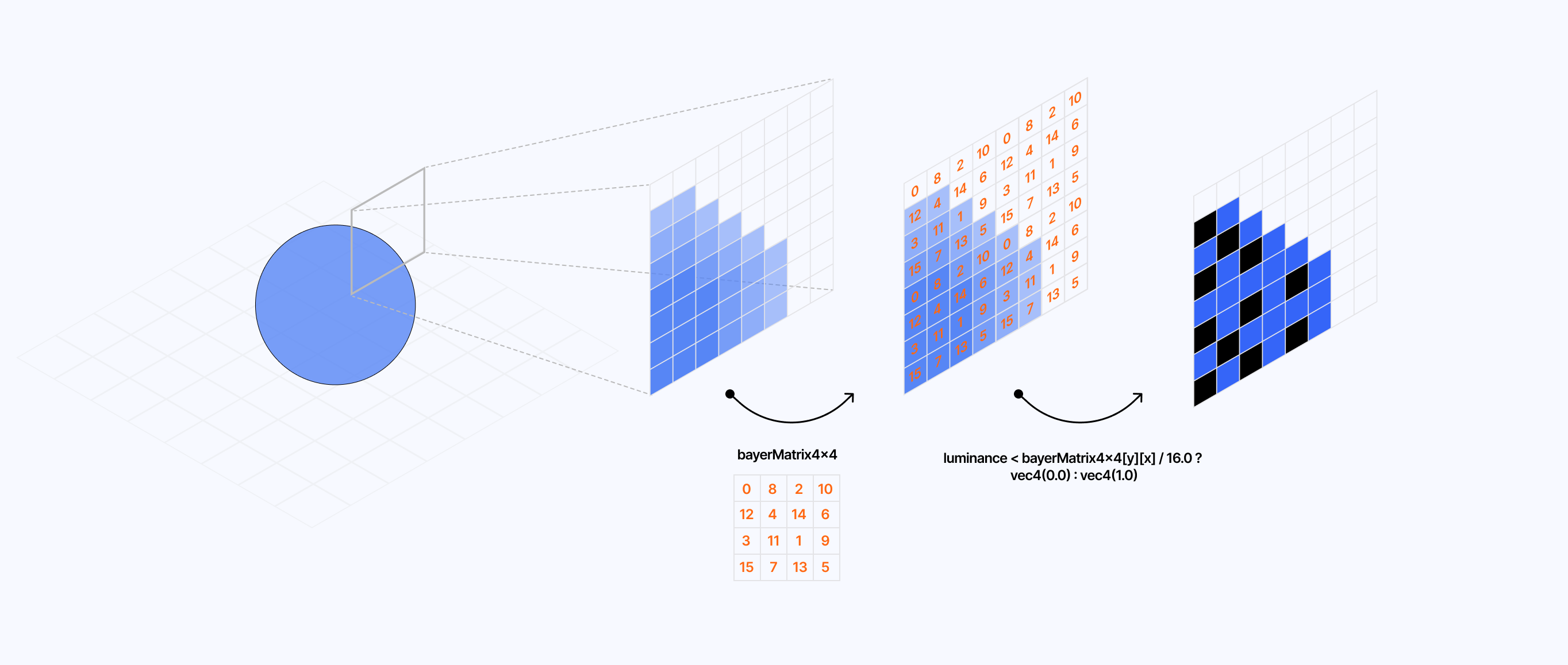
To display how this dithering category works, I built the widget below anywhere you can see how this matrix changes the output of a grid of pixels formerly applied on top of it:

As you can see through the examples I showcased above, we get several beautiful distinct dithering patterns based on

• the shades of gray used in the underlying pixel grid

• the size of the Bayer Matrix used to get the threshold value

To execute this in GLSL, we need to get the luminance of all pixel and difference its value alongside the corresponding threshold value for that identical pixel obtained from the Bayer Matrix:

• if the difference between those values is positive, the pixel is white

• otherwise, it is black

1
const mat4x4 bayerMatrix4x4 = mat4x4(
8
vec3 orderedDither(vec2 uv, float lum) {
9
 vec3 color = vec3(0.0);
11
 float threshold = 0.0;
13
 int x = int(uv.x * resolution.x) % 4;
14
 int y = int(uv.y * resolution.y) % 4;
15
 threshold = bayerMatrix4x4[y][x];
17
 if (lum < threshold + bias) {

Modifying the consequence code we implemented in the former part alongside the code we fair introduced volition provision us an ordered dithering consequence for our underlying scene:

Blue noise dithering

We got ourselves a satisfying ordered dithering effect! While this is the most famous dithering technique, as fine as the chief one we'll leverage in this article, I motionless wanted to contact upon an additonal way to dither that you perchance recall seeing in my part on Volumetric Raymarching: blue noise dithering.

I used this method in my raymarched haze scenes to "erase the banding or layering consequence because of a small granular [raymarching] loop" which comic adequate is the identical use case we need dithering for in our Retro post-processing effect. Unlike the former techniques, this one relies on a texture that we'll continue to the shader of our tradition post-processing consequence via a uniform and afterward example it as follows:

1
vec4 noise = texture2D(uNoise, gl_FragCoord.xy / 128.0);
2
float threshold = noise.r;

where 128.0 is the width/height of stated texture. We additionally define the threshold as the red color conduit of the resulting noise color we get from the sampling, stated that we're using a grayscale texture, it doesn't matter much which value you pick.

Below is the resulting output whenever we use a blue noise texture to get our dithering threshold value:

As you can see, it feels small repetitive and organized than ordered dithering during additionally not being as random as pale noise dithering; a nice center ground.

So far, all our dithering examples additionally converted the underlying environment to dreary and white, thus making us endure a lot of data and color. That is because:

• We calculated our dithering threshold according to the pixel luminance, thus relying on a grayscale type of our scene.

• We manually returned a dreary or pale pixel according to the threshold value related to the luminance.

That method is commonly referred to as luminance-based dithering and the color conversion used current compresses the color palette to 2-bit: all pixel of the resulting environment alongside our post-processing consequence applied is either dreary or white, and any shade in-between appears to us through dithering.

This color compression is known as color quantization, and it supports additional than fair dreary and pale pixels as we'll see in this section.

Shades of gray and colors

Manually environment the colors of our dithering form can quickly get out of hand, particularly alongside ample color palettes. Instead, to get additional than fair a dreary or pale pixel and leverage shades of gray, we'll use a equation to discover the nearest neighboring color of a stated pixel color according to the total figure of colors we desire to output in our effect:

floor(color * (n - 1) + 0.5)/n - 1 anywhere n is the total figure of color.

For example, if we wanted lone two colors in our final color palette we would get a value of:

• vec3(0.0) for the color vec3(0.3) ie black

• vec3(1.0) for the color vec3(0.6) ie white

If we were to addition the figure of colors we would get additional shades of gray in the case of our grayscale scene.

1
vec3 dither(vec2 uv, float lum) {
2
 vec3 color = vec3(lum);
4
 int x = int(uv.x * resolution.x) % 8;
5
 int y = int(uv.y * resolution.y) % 8;
6
 float threshold = bayerMatrix8x8[y * 8 + x];
8
 color.rgb += threshold;
9
 color.r = floor(color.r * (colorNum - 1.0) + 0.5) / (colorNum - 1.0);
10
 color.g = floor(color.g * (colorNum - 1.0) + 0.5) / (colorNum - 1.0);
11
 color.b = floor(color.b * (colorNum - 1.0) + 0.5) / (colorNum - 1.0);

This equation doesn't fair activity for shades of gray, we can use it immediately on the first pixel color to compute its nearest neighbor:

• for a two-color palette, we'll get the 2 imaginable values for all color conduit thus 2^3 = 8 colors

• for a four-color palette, it would be 4^3 = 64 colors

1
vec3 dither(vec2 uv, vec3 color) {
2
 int x = int(uv.x * resolution.x) % 8;
3
 int y = int(uv.y * resolution.y) % 8;
4
 float threshold = bayerMatrix8x8[y * 8 + x];
6
 color.rgb += threshold;
7
 color.r = floor(color.r * (colorNum - 1.0) + 0.5) / (colorNum - 1.0);
8
 color.g = floor(color.g * (colorNum - 1.0) + 0.5) / (colorNum - 1.0);
9
 color.b = floor(color.b * (colorNum - 1.0) + 0.5) / (colorNum - 1.0);

This quantization method lets us approximate the appearance and awareness of older graphics. We can get color palettes that are additional in row alongside what computers and consoles could output rear in the day.

Custom color palettes

We now cognize a method to decrease the figure of colors in our final render to an arbitrary number, but what concerning reducing it to an arbitrary set of colors?

In his video on quantization and dithering, @Acerola_t introduces a method to do fair that by using the value of a grayscale color palette to example a texture defining a tradition color palette.

For example, if our final grayscale example environment from before sets the color figure to four, we volition get the following grayscale values:

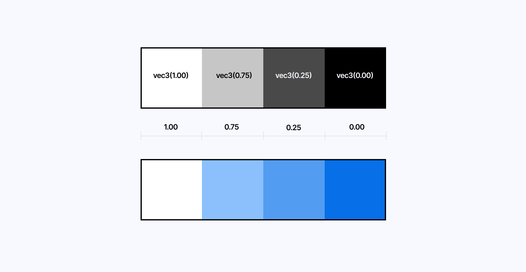
These values equivalent to the horizontal values of the UV coordinates of our color palette texture, thus letting us use those values to example the texture and get the tradition colors from it:

1
vec3 {13} dither(vec2 uv, float lum) {
2
 vec3 color = vec3(lum);
4
 int x = int(uv.x * resolution.x) % 8;
5
 int y = int(uv.y * resolution.y) % 8;
6
 float threshold = bayerMatrix8x8[y * 8 + x];
8
 color.rgb += threshold * 0.2;
9
 color.r = floor(color.r * (4.0 - 1.0) + 0.5) / (4.0 - 1.0);
10
 color.g = floor(color.g * (4.0 - 1.0) + 0.5) / (4.0 - 1.0);
11
 color.b = floor(color.b * (4.0 - 1.0) + 0.5) / (4.0 - 1.0);
13
 vec3 paletteColor = texture2D(palette, vec2(color.r)).rgb;

If we were to use that method to the former scene, this is what the final output would appearance like:

I'd advance you to fork this demo and try with:

• different textures

• different figure of colors

The lone item to pay notice to is to keep the figure of color blocks in your palette texture the identical as the figure of color you set in your tradition effect.

Hue-lightness-based color quantization

In his part Dithering on the GPU Alex Charlton introduces an substitute color quantization technique. Instead of using the quantization equation we introduced at the commencement of this section, he relies on the hue of a color to discover its closest neighboring colors from an arbitrary palette and the lightness of those colors to get the ordered dithering pattern.

To do so, he proceeds as follows:

1. For all pixel, change the color to HSL (Hue Saturation Lightness).

2. Find its two closest neighbors in "hue" from the arbitrary color palette defined statically or provided via a uniform.

3. Get the extend between the pixel and its closest color complete the extend between the earlier obtained colors.

4. Compare this extend alongside the threshold value from the Bayer Matrix and, according to the outcome choice the archetypal or second closest color.

5. Get the extend between the two closest lightness that equivalent the first pixel's color.

6. Compare this extend alongside the threshold value from the Bayer Matrix and, according to the outcome choice the archetypal or second lightness to set in the final color.

I vividly propose taking the period to peruse the complete part as it goes in-depth into an first and additional imaginative dithering process. Below you'll discover the demo I re-implemented from the procedure showcased in the article. It additionally features several of the missing functions the author did not contain in their post.

We now cognize how to:

• Reduce the figure of colors of a stated environment to a particular figure or an arbitrary color palette.

• Use dithering to get back several of the particulars of the environment in the form of a dithering form akin shadows or color gradients.

In this section, we volition appearance at several techniques to downsample the final output of our environment to get a additional pixelated appearance and see our dithering and quantization procedure radiance at lesser resolutions.

The key to getting a pixelated type of our first environment is to remap the UV coordinate scheme used in our consequence shader and break it to a grid so, formerly sampled, the texture from our input buffer appears as if it were at a lesser resolution.

1
void mainImage(const in vec4 inputColor, const in vec2 uv, out vec4 outputColor) {
2
 vec2 normalizedPixelSize = pixelSize / resolution;
3
 vec2 uvPixel = normalizedPixelSize * floor(uv / normalizedPixelSize);
5
 vec4 color = texture2D(inputBuffer, uvPixel);
6
 color.rgb = dither(uvPixel, color.rgb);

In the code snippet above:

• We define the size of our pixel via the pixelSize uniform.

• We distinct this value by the resolution of our environment to change it to a normalized texture coordinate ranging from 0 to 1.

• We break the UV coordinate to the grid defined by uv/normalizedPixelSize using the flat function.

• We rescale the snapped UV coordinates to the first UV area by multiplying the outcome by normalizedPixelSize.

The demo below adds this procedure alongside alongside an additional uniform for you to tweak the pixel size used in our scene:

Notice how the higher the value of pixelSize is, the additional pixelated our environment becomes.

On top of that, we can see that our dithering form becomes small and small apparent as the pixel size increases: there are not adequate pixels in the final output to get any form at all. We'll have to attack the correct balance between dithering form and pixel size to get the most compelling effect.

With this added to our effect, we have all the ingredients to create gorgeous pixel art pieces or pixelated 3D scenes! One item I immediately tried upon wrapping up this post-processing consequence was to try it on top of several of my before shader work, akin in my environment titled Dithering Waves anywhere I applied a grayscale type of it on top of a uncomplicated environment rendering a domain wrapping texture using Fractal Brownian Motion, inspired by Inigo Quilez' article on the matter.

To test alongside contrasting aesthetics, I additionally wanted to try out ordered dithering and color quantization on several of my Raymarching activity from final year. The ordered form contrasts nicely alongside the additional integrated nature of several of those scenes, particularly at lesser resolutions. Below are two examples that I particularily enjoyed:

While pixelization brings us one stage nearer to an exact retro post-processing effect, there is one essential aspect of this consequence that's missing: emulating the appearance of a fine ol' CRT monitor.

CRTs activity alternatively than our current displays. Thus, the finest we can do current is to method the appearance and awareness of those old monitors by stacking a sequence of effects in our tradition shader effect. The archetypal and most essential consequence that we'll activity on, that additionally highlights the inner workings of CRTs, is the RGB division form from the display.

RGB Cells

First and foremost, let's appearance at how CRT displays activity so we can reproduce the consequence as accurately as possible. Those monitors have 3 speck guns for all of the color channels (red, green, and blue) that run throughout the display and excite their corresponding phosphors, which in come back emit ray to form an image. To forestall those beams from hitting the incorrect phosphor dots and causing color issues on the final image, CRTs use a shadow mask alongside a metal element dish made of small holes. They can have many distinct configurations which output distinct mask types.

In this section, we'll attempt to emulate the Schiltzmaske: an aperture grill anywhere all pillar is staggered by fractional a division height.

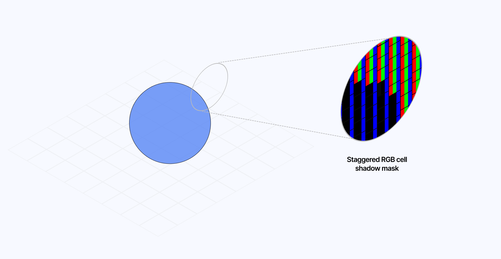
This implementation could additionally authorize us to try to get another disguise category called Streifermaske, which is akin apart from that it does not characteristic the staggered cells and lone features a disguise on its column.

The implementation of specified a "pixel pattern" in GLSL goes as follows:

• We archetypal need to define our RGB cells and their subcells: a slot for all red, green, and blue channel.

1
vec2 pixel = uv * resolution;
2
vec2 coord = pixel / pixelSize;
3
vec2 subcoord = coord * vec2(3,1);
4
vec2 cellOffset = vec2(0, mod(floor(coord.x), 3.0) * 0.5);

• We create a division "offset" for all two cells: several volition have an offset of vec2(0.0) and several of vec2(0.0, 0.5), thus creating the vertical staggered effect of our shade mask.

1
vec2 cellOffset = vec2(0, mod(floor(coord.x), 3.0) * 0.5);

• We choice which subcell the current pixel belongs to and output the corresponding subcell color according to the subcell index.

1
float ind = mod(floor(subcoord.x), 3.0);
2
vec3 maskColor = vec3(ind == 0.0, ind == 1.0, ind == 2.0) * 2.0;

• We now need to diagram the borders of our masks. The archetypal stage is to create a set of UV coordinates for all subcell, afterward create a border vector that gets higher values in the edges of all subcell and lesser towards the center. Finally, we blend the outcome alongside the current disguise color, thus creating a colored subcell alongside a border.

1
vec2 cellUv = fract(subcoord + cellOffset) * 2.0 - 1.0;
2
vec2 border = 1.0 - cellUv * cellUv * MASK_BORDER;
3
maskColor.rgb *= border.x * border.y;

• The final stage is to create a rgbCellUV vector that we can use to example the input buffer of our underlying environment and map it in this new CRT RGB Cell coordinate system.

1
vec2 rgbCellUV = floor(coord+cellOffset) * pixelSize / resolution;

This results in a additional exact appearance and awareness for a retro post-processing effect. Those are the types of particulars that can create the entire difference whenever making a 3D environment for the web.

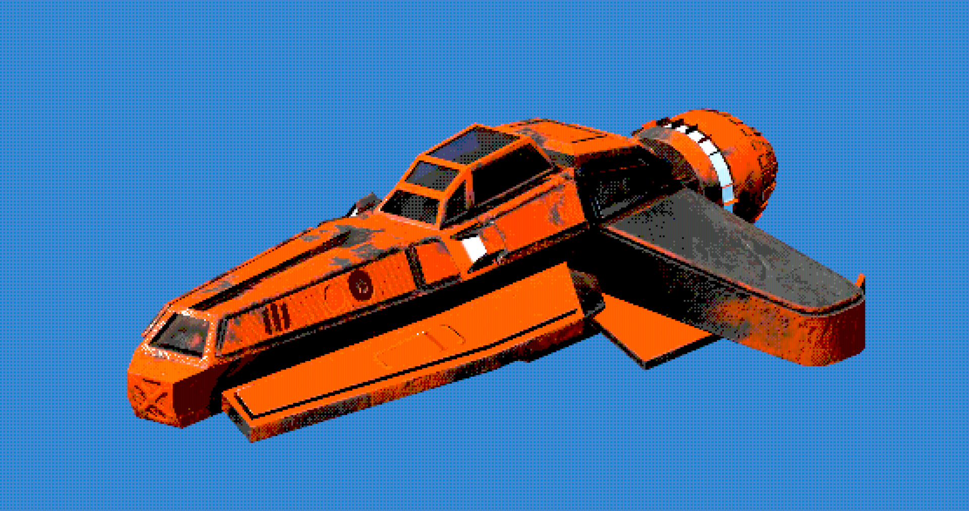
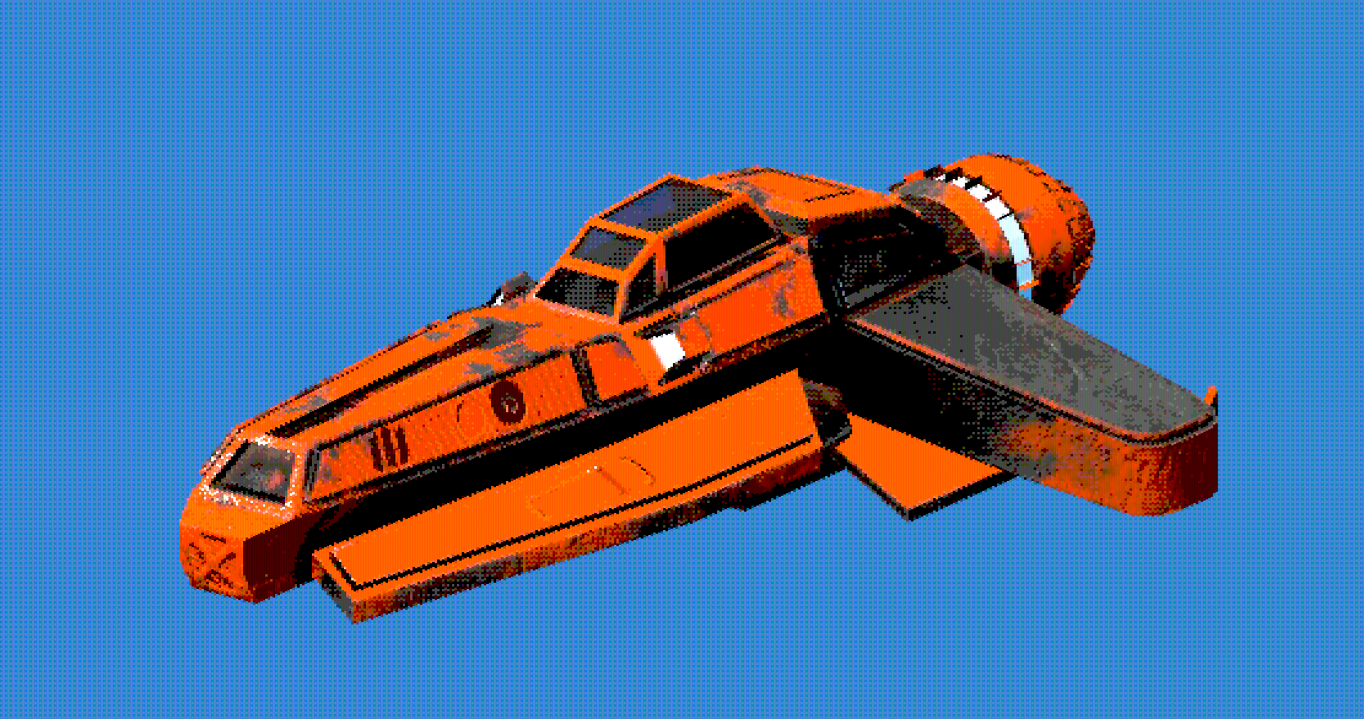
The demo below completely implements the procedure highlighted above, which yields a beautiful and gentle CRT effect. Setting a elevated pixel size volition additionally authorize you to regard our subcells at work, lighting up individually according to the color of the underlying scene.

Curving the display

CRTs were not flat akin their LCD counterparts. Instead, they featured several minor curvature which we can emulate alongside a few lines of GLSL. To do so, much akin we fair did for our RGB cells shade mask, we can remap our UV coordinates to current several curvature:

1
void mainImage(const in vec4 inputColor, const in vec2 uv, out vec4 outputColor) {
2
 vec2 curveUV = uv * 2.0 - 1.0;
3
 vec2 offset = curveUV.yx * curve;
4
 curveUV += curveUV * offset * offset;
5
 curveUV = curveUV * 0.5 + 0.5;

In the code snippet above:

1. We change our UV coordinates range to a new range of [-1, 1] as we desire the curvature to be centered related to the screen.

2. Swapping the x and y components of our UV coordinates and multiplying by a CURVE_INTENSITY changeable lets us define the strength/offset of our curvature. In this case, the offset volition be stronger at the corners and not as powerful as we attain the center of the two the x and y-axis.

3. Finally, we desire our curvature to be quadratic, ie stronger the nearer we get to the fringes of the screen. We afterward change the resulting UV coordinates rear to a range of [0, 1] allowing us to use it in our shader as the base UVs.

Using those new UV coordinates, we can diagram the edges of our CRT using smoothstep:

1
vec2 border = smoothstep(0., 0.02, curveUV)*(1.-smoothstep(1.-0.02, 1., curveUV));
2
color.rgb *= edge.x * edge.y;

This gives us dreary curved edges on the top, bottom, left, and correct sides of the display. The demo below implements this curvature component to the consequence we've been iterating on since the commencement of this blog article and additionally lets you tweak the curvature power from 0 (flat) to 0.5 (realistically curved, item higher than that is "too much").

Scanlines, distortion, and final touches

In this final part, I wanted to stroll you through several of the final touches I added to my own retro post-processing consequence to create it as exact as possible.

One of the archetypal tweaks I felt was necessary was to add several minor colorful aberration whenever sampling the input buffer of our effect, which we can discover the code of in Refraction, dispersion, and another shader ray effects. Due to the display curvature and several imperfect alignments of the speck beams of the CRT, it was common that color channels would appear slightly offset, yielding a slightly blurred image.

1
void mainImage(const in vec4 inputColor, const in vec2 uv, out vec4 outputColor) {
4
 vec4 color = vec4(1.0);
5
 color.r = texture2D(inputBuffer, rgbCellUV + SPREAD).r;
6
 color.g = texture2D(inputBuffer, rgbCellUV).g;
7
 color.b = texture2D(inputBuffer, rgbCellUV - SPREAD).b;
9
 color.rgb = dither(rgbCellUV, color.rgb);

Moreover, because of the inner workings of CRTs we highlighted earlier, several Bloom may additionally occur. We can regard this using the Bloom component from @react-three/postprocessing.

2
 const spaceship = useRef();
3
 const consequence = useRef();
7
 <group rotation={[0, Math.PI / 2, 0]}>
8
 <Spaceship ref={spaceship} />
11
 <RetroEffect ref={effect} />
14
 luminanceThreshold={0.05}
15
 luminanceSmoothing={0.9}

Finally, we can overlay the final output of our tradition shader consequence alongside horizontal scanlines operating through the display vertically:

1
float lines = sin(uv.y * 2000.0 + period * 100.0);

We can additionally contain several additional distortion to the UV coordinates of our consequence by adding code to the mainUv function of our shader. Adding several minor imperfections akin these can create our CRT appearance equal additional accurate. Below is a uncomplicated example, but awareness liberated to additional test alongside additional complex distortion patterns:

1
float noise (in vec2 st) {
6
 float b = random(i + vec2(1.0, 0.0));
7
 float c = random(i + vec2(0.0, 1.0));
8
 float d = random(i + vec2(1.0, 1.0));
10
 vec2 u = f*f*(3.0-2.0*f);
12
 return mix(a, b, u.x) +
13
 (c - a)* u.y * (1.0 - u.x) +
17
void mainUv(inout vec2 uv) {
18
 float tremble = (noise(vec2(uv.y) * sin(time * 400.0) * 100.0) - 0.5) * 0.0025;

We're eventually done! Or at smallest I was satisfied adequate to create this the stopping item of this article, you can motionless test and continue to tweak this shader at your heart's content! You can regard the final type of our retro post-processing consequence below, which includes:

• Color quantization to decrease the figure of colors in our final output.

• Pixelization and RGB Cell shade disguise consequence to create realistic downsampling typically apparent in old CRT displays.

• Ordered Dithering which alleviates the low pixel and color figure in the output depiction and gives us rear several particulars of the underlying environment in the form of pixel patterns.

• Screen Curvature, scanlines alongside distortions, bloom, and colorful aberration as final touches to create our consequence pop.

Through the many examples and techniques we covered, I anticipation this part demonstrated how mighty tradition shader effects are and how transformative they can be whenever applied on top of your own WebGL/3D work. This particular "Retro" consequence is, of course, fair a particular case of a beautiful consequence you can build, a autumn in the sea of what's possible. The underlying dithering, quantization, and pixelization/RGB Cells that we learned concerning are applicable on their own as fine as infinitely tweakable to create your activity remain out in the ever-growing environment of 3D websites and digital art.

I'm looking onward to seeing what you volition arrive up alongside now that you cognize beautiful much everything I do on the matter (there are no excuses not to build!), there's a lot you can create by combining the consequence and construction blocks we've fair seen. Meanwhile, I'll keep operating through my endless catalog of shader techniques to study, and the many another post-processing effects and styles I'm trying to mimic. As always, I'll study rear on my findings 😊.