
Introduction
Part 2: Knowledge Distillation, KV Caching, and Speculative Decoding
In Part 1, we saw really quantization reduces the numerical precision of exemplary weights and really pruning removes redundant connections, some techniques that target the model itself earlier it ever sees a request.
Part 2 takes a different angle. The 3 techniques covered present optimize exemplary conclusion from different directions: Knowledge Distillation trains a smaller, faster exemplary to behave for illustration a larger one. KV Caching eliminates redundant computation astatine runtime by storing and reusing intermediate attraction states. Speculative Decoding parallelizes what is, by design, a sequential process, frankincense making the GPU do aggregate tokens’ worthy of activity successful the clip it would usually do one.
Together, they correspond the astir impactful techniques for making LLMs accelerated and deployable successful production, and not conscionable making them a theoretical concept, but really responsive astatine scale.
By the extremity of this article, we will study really each method useful astatine the algorithm level, wherever they fresh successful a existent conclusion pipeline, and really they constitute pinch the techniques from Part 1 to build a afloat optimized serving stack.
Key Takeaways
- Knowledge Distillation transfers the “soft knowledge” encoded successful a ample model’s probability distributions into a smaller student exemplary — not conscionable the last answers. Instead of learning only the last prediction, the smaller exemplary besides learns from the assurance levels the larger exemplary assigns to different tokens. This helps the smaller exemplary execute amended than its size would usually suggest.
- KV Caching is the azygous astir impactful runtime optimization successful modular LLM serving. Without it, generating each caller token requires recomputing attraction complete the full discourse from scratch — an O(n²) operation. With it, we only process the caller token.
- PagedAttention solves KV cache fragmentation — the hidden representation discarded from over-allocating cache abstraction for sequences that ne'er scope max length. It’s the halfway invention down vLLM’s throughput advantages.
- Speculative Decoding exploits an asymmetry: verifying K campaigner tokens successful parallel is cheaper than generating K tokens sequentially. A accelerated draught exemplary speculates; the ample exemplary verifies — and we get the nonstop aforesaid output distribution arsenic moving the ample exemplary alone, conscionable faster.
- EAGLE-2 and Medusa bring speculative decoding into accumulation without requiring a abstracted draught exemplary — making the method accessible moreover erstwhile we are deploying a azygous model.
Knowledge Distillation
The Core Idea
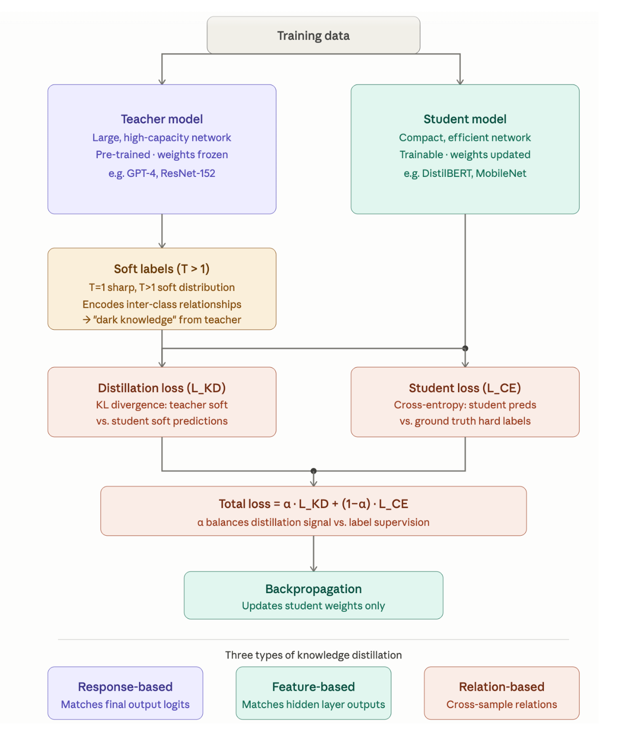
Imagine location is simply a professor who knows everything, and a student who needs to walk the aforesaid exam. The naive approach: springiness the student the aforesaid textbooks and dream for the best. The smarter approach: person the professor explicate why each reply is right, not conscionable what the reply is.
That’s knowledge distillation successful 1 sentence. The “professor” is simply a large, powerful teacher model. The “student” is simply a smaller, faster student model. The extremity isn’t conscionable to get the student to nutrient the aforesaid outputs but alternatively to get the student to sorb the aforesaid reasoning patterns encoded successful the teacher’s probability distributions.
Why Probability Distributions Carry More Information Than Labels
When a coach exemplary assigns probabilities to tokens, the distribution itself is informative. If the coach outputs:
“dog”: 0.72, “wolf”: 0.18, “cat”: 0.06, “fox”: 0.04
This tells the student acold much than the difficult explanation "dog". It says: dog and wolf are semantically related, this is simply a adjacent call, and feline and fox are plausible but distant. A student trained only connected difficult labels would ne'er spot that signal.
This is the cardinal penetration of Hinton et al.'s 2015 distillation paper: soft labels are richer supervisory signals than difficult labels.
The Loss Function
The training nonsubjective combines 2 losses:
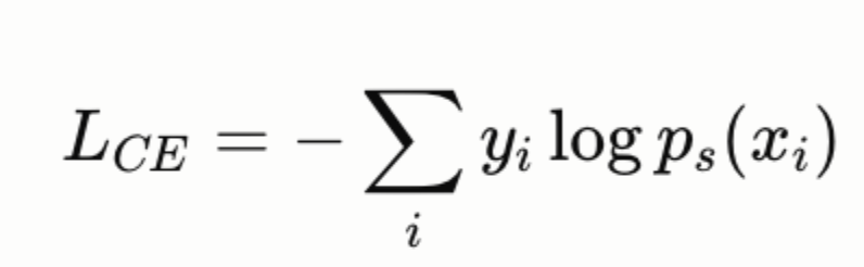
Cross-entropy loss connected difficult labels (standard supervised learning):
KL divergence loss betwixt coach and student distributions, computed astatine somesthesia T:

The facet T² compensates for the truth that soft targets astatine precocious somesthesia person smaller gradients. The mixed nonaccomplishment is:
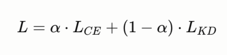
where α controls really overmuch weight we springiness to crushed truth labels vs. coach guidance. In practice, α = 0.1–0.5 useful good — we want the teacher’s awesome to dominate.
Temperature T > 1 softens the teacher’s distribution, making it little peaked. This amplifies the awesome successful the smaller probability values (the “dark knowledge”) that would different beryllium drowned retired by the ascendant token’s probability. A emblematic worth is T = 2–4.
Distillation Flavors
Response-Based Distillation is the simplest: the student learns from the teacher’s last output logits. No entree to the teacher’s internals is needed. This is what DistilBERT and TinyLLaMA use.
Feature-Based Distillation goes deeper. The student is besides trained to mimic the teacher’s intermediate hidden states — the activations astatine circumstantial layers. The intuition: a layer’s hidden authorities encodes its learned practice of the input. If the student’s hidden states look for illustration the teacher’s, the student has internalized not conscionable what to predict, but really to logic astir the input.
The nonaccomplishment for a fixed furniture brace (student furniture s, coach furniture t) is:
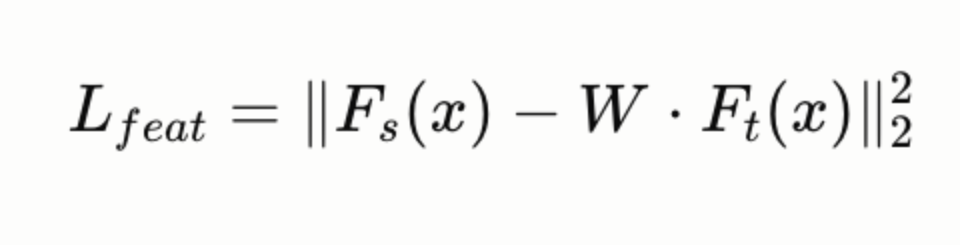
where W is simply a learned projection matrix that maps coach characteristic dimensions to student characteristic dimensions (necessary erstwhile they differ).
Relation-Based Distillation transfers pairwise relationships betwixt samples — alternatively than matching individual activations, the student learns to sphere the similarity building of the teacher’s practice space.
Patient Knowledge Distillation (PKD)
Standard distillation only uses the teacher’s last layer. PKD proposes utilizing multiple intermediate layers of the coach arsenic supervision signals. The student “patiently” learns from each furniture of the teacher, not conscionable the output.
This is peculiarly effective for BERT-style encoders, wherever intermediate representations encode progressively absurd linguistic features. A student trained pinch PKD converges faster and retains much of the teacher’s soul knowledge astatine little parameter counts.
MiniLLM: Fixing the Mode-Averaging Problem
Forward KL divergence (used successful modular distillation) minimizes:
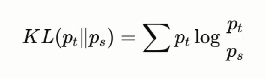
This penalizes the student heavy erstwhile p_s is small, but p_t is ample — meaning the student is forced to screen each the modes of the teacher’s distribution, including low-probability ones. For autoregressive matter generation, this causes mode averaging: the student spreads probability wide crossed galore plausible continuations, producing generic, hedging outputs.
MiniLLM flips the direction:
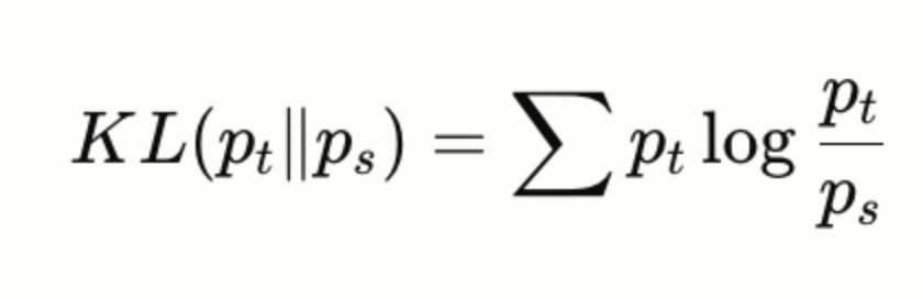
Reversed KL penalizes the student for putting probability wide wherever the coach doesn’t — it encourages mode-seeking alternatively than mode-covering. The student learns to prime the astir confident, high-quality continuations alternatively than averaging crossed each plausible ones.
MiniLLM besides addresses exposure bias: during modular training, the student ever sees ground-truth prefixes, but astatine inference, it conditions connected its ain outputs. MiniLLM uses argumentation gradient optimization complete the student’s ain generated sequences, which closes this train-inference gap.
Python Example: Teacher-Student Distillation Training Loop
import torch import torch.nn as nn import torch.nn.functional as F from transformers import AutoModelForCausalLM, AutoTokenizer from torch.utils.data import DataLoader class DistillationTrainer: def __init__( self, teacher_model, student_model, temperature: float = 2.0, alpha: float = 0.5, device: str = "cuda" ): self.teacher = teacher_model.to(device).eval() self.student = student_model.to(device) self.T = temperature self.alpha = alpha self.device = device # Freeze coach — it's a fixed oracle for param in self.teacher.parameters(): param.requires_grad = False def distillation_loss(self, student_logits, teacher_logits, labels): """ Combines hard-label cross-entropy pinch soft-label KL divergence. student_logits: [batch, seq_len, vocab_size] teacher_logits: [batch, seq_len, vocab_size] labels: [batch, seq_len] — crushed truth token IDs """ # --- Hard explanation nonaccomplishment (standard connection modeling) --- # Shift truthful that token n predicts token n+1 shift_logits = student_logits[..., :-1, :].contiguous() shift_labels = labels[..., 1:].contiguous() L_ce = F.cross_entropy( shift_logits.view(-1, shift_logits.size(-1)), shift_labels.view(-1), ignore_index=-100 ) # --- Soft explanation nonaccomplishment (KL divergence astatine somesthesia T) --- # Apply somesthesia scaling to some coach and student soft_teacher = F.softmax(teacher_logits[..., :-1, :] / self.T, dim=-1) soft_student = F.log_softmax(student_logits[..., :-1, :] / self.T, dim=-1) # T^2 scaling compensates for reduced gradient magnitudes astatine precocious T L_kd = (self.T ** 2) * F.kl_div( soft_student, soft_teacher, reduction="batchmean" ) # Combined loss return self.alpha * L_ce + (1 - self.alpha) * L_kd def train_step(self, input_ids, attention_mask, optimizer): input_ids = input_ids.to(self.device) attention_mask = attention_mask.to(self.device) # Teacher guardant walk (no gradients needed) with torch.no_grad(): teacher_out = self.teacher( input_ids=input_ids, attention_mask=attention_mask ) teacher_logits = teacher_out.logits # Student guardant walk (gradients travel here) student_out = self.student( input_ids=input_ids, attention_mask=attention_mask ) student_logits = student_out.logits # Compute distillation loss nonaccomplishment = self.distillation_loss(student_logits, teacher_logits, input_ids) # Backprop connected student only optimizer.zero_grad() loss.backward() optimizer.step() return loss.item() def run_distillation(teacher_name, student_name, dataset, epochs=3, lr=1e-4): """ Example: distill Mistral-7B → TinyLLaMA-1.1B """ coach = AutoModelForCausalLM.from_pretrained(teacher_name, torch_dtype=torch.float16) student = AutoModelForCausalLM.from_pretrained(student_name, torch_dtype=torch.float32) trainer = DistillationTrainer( teacher_model=teacher, student_model=student, temperature=2.0, alpha=0.3 # 30% difficult labels, 70% coach guidance ) optimizer = torch.optim.AdamW(student.parameters(), lr=lr) dataloader = DataLoader(dataset, batch_size=4, shuffle=True) for epoch in range(epochs): total_loss = 0.0 for batch in dataloader: nonaccomplishment = trainer.train_step( input_ids=batch["input_ids"], attention_mask=batch["attention_mask"], optimizer=optimizer ) total_loss += loss avg_loss = total_loss / len(dataloader) print(f"Epoch {epoch+1}/{epochs} | Loss: {avg_loss:.4f}") return studentDistillation is the correct instrumentality erstwhile we request a exemplary mini capable to tally connected separator hardware, aliases inexpensive capable to service astatine scale, but we can’t spend to commencement from scratch. Common scenarios: a 1.1B exemplary distilled from LLaMA-2-7B for on-device inference; domain-specific distillation wherever a fine-tuned 13B coach transfers domain expertise into a 1B student; aliases capacity distillation for constrictive tasks for illustration SQL procreation aliases codification completion, wherever a ample wide exemplary teaches a mini specialized one.
Importantly, distillation and quantization constitute cleanly. The emblematic pipeline is: distill first (model compression), past quantize (weight compression), past deploy pinch the runtime optimizations below.
KV Cache
Why Attention Has a Memory Problem
To understand KV caching, we first request to understand what happens during autoregressive matter procreation without it.
In a transformer’s attention mechanism, for each token position i, the exemplary computes 3 vectors: Query (Q), Key (K), and Value (V). The attraction output astatine position one is:

Here, K and V span each erstwhile positions — the exemplary attends to its full discourse to determine what the adjacent token should be.
Now see what happens erstwhile we make token 101. We request K and V for tokens 1 done 100. Then, for token 102, we request K and V for tokens 1 done 101. If we are not caching, we are recomputing K and V for tokens 1–100 from scratch each azygous step. That’s O(n) redundant computation per token, starring to O(n²) total, and it gets worse arsenic sequences turn longer.
KV caching simply stores the K and V matrices arsenic we compute them and appends to the cache pinch each caller token. At measurement n, we only compute K, V for the caller token, past concatenate pinch the cache. Suddenly, attraction complete agelong contexts is O(1) per step.
The Memory Cost of Caching
KV cache is not free — it trades compute for memory. The cache size for a azygous series is:

where L is the number of layers, H is the number of KV heads, d_h is caput dimension, s is series length, and b is bytes per element.
For LLaMA-2-7B astatine FP16 (2 bytes per element):
- L = 32 layers, H = 32 heads, d_h = 128, astatine series magnitude 4096
- KV cache = 2 × 32 × 32 × 128 × 4096 × 2 = 4.29 GB
That’s conscionable for 1 sequence. At a batch size of 16, we are looking astatine 68 GB of KV cache unsocial — earlier moreover fitting the exemplary weights.
This is why the architecture of attraction heads matters enormously for conclusion efficiency.
Multi-Head vs Multi-Query vs Grouped-Query Attention
These 3 attraction variants correspond different trade-offs betwixt value and KV cache size:
Multi-Head Attention (MHA) — the original transformer design. Each attraction caput has its ain independent K and V projections. For H heads, we shop H × 2 matrices per layer. Maximum expressiveness, maximum representation cost.
Multi-Query Attention (MQA) — each H attraction query heads stock a single K caput and a single V head. Reduces KV cache by a facet of H (typically 8–32×). The catch: value degrades, particularly connected tasks requiring divers attraction patterns. Used successful PaLM, Falcon.
Grouped-Query Attention (GQA) — a mediate ground. Query heads are divided into G groups, each group sharing 1 K and 1 V head. With G groups, the KV cache is reduced by H/G. LLaMA-2-70B uses G=8 (from 64 query heads, 8 KV heads), reducing KV cache by 8× pinch minimal value loss. LLaMA-3 and Mistral usage GQA crossed each exemplary sizes.
MHA: [Q1,Q2,...,QH] → [K1,K2,...,KH], [V1,V2,...,VH] # H KV pairs GQA: [Q1..Q8] → [K1,V1], [Q9..Q16] → [K2,V2], ... # G KV pairs (G << H) MQA: [Q1..QH] → [K1,V1] # 1 KV pairPagedAttention: Solving the Fragmentation Problem
Even pinch GQA reducing cache size, naive KV cache guidance wastes memory. The modular attack reserves max_seq_len contiguous blocks of GPU memory for each series astatine petition start. If max_seq_len is 4096 but the existent consequence is 200 tokens, we person wasted 3896 tokens’ worthy of cache. With hundreds of concurrent requests, this fragmentation causes GPU representation utilization of 20–40%.
PagedAttention, the halfway invention successful vLLM, borrows the solution from the operating strategy virtual memory: paging.
Instead of contiguous pre-allocation, PagedAttention divides the KV cache into fixed-size blocks (pages), each holding K and V for a fixed number of tokens (e.g., 16). A block table maps each sequence’s logical positions to beingness blocks. Blocks are allocated connected request arsenic the series grows, and freed instantly erstwhile the series completes.
The result: GPU representation utilization supra 90%, enabling 2-4× higher throughput compared to naive implementations. vLLM besides uses paging to alteration copy-on-write for parallel sampling — aggregate consequence candidates stock the aforesaid KV cache blocks for the prompt, pinch blocks only duplicated erstwhile their contented diverges.
Python Example: KV Cache successful Attention
Here’s a minimal implementation showing really KV caching useful successful a multi-head attraction furniture — the mechanics vLLM and different frameworks build on:
import torch import torch.nn as nn import torch.nn.functional as F from dataclasses import dataclass, field from typing import Optional, Tuple @dataclass class KVCache: """ Stores accumulated Key and Value tensors crossed procreation steps. Shape: [batch, n_heads, seq_len, head_dim] """ keys: Optional[torch.Tensor] = None values: Optional[torch.Tensor] = None def update(self, new_keys: torch.Tensor, new_values: torch.Tensor): """Append caller K, V to the cache on the series dimension.""" if self.keys is None: self.keys = new_keys self.values = new_values else: self.keys = torch.cat([self.keys, new_keys], dim=2) # dim=2 is seq_len self.values = torch.cat([self.values, new_values], dim=2) return self.keys, self.values @property def seq_len(self) -> int: return self.keys.shape[2] if self.keys is not None else 0 class CachedMultiHeadAttention(nn.Module): def __init__(self, d_model: int, n_heads: int): super().__init__() assert d_model % n_heads == 0 self.n_heads = n_heads self.head_dim = d_model // n_heads self.scale = self.head_dim ** -0.5 self.q_proj = nn.Linear(d_model, d_model, bias=False) self.k_proj = nn.Linear(d_model, d_model, bias=False) self.v_proj = nn.Linear(d_model, d_model, bias=False) self.o_proj = nn.Linear(d_model, d_model, bias=False) def _split_heads(self, x: torch.Tensor) -> torch.Tensor: """[batch, seq, d_model] → [batch, n_heads, seq, head_dim]""" B, S, D = x.shape return x.view(B, S, self.n_heads, self.head_dim).transpose(1, 2) def forward( self, x: torch.Tensor, # [B, seq_len, d_model] — existent token(s) kv_cache: Optional[KVCache] = None, use_causal_mask: bool = True ) -> Tuple[torch.Tensor, KVCache]: B, S, _ = x.shape # Project Q, K, V for the existent input Q = self._split_heads(self.q_proj(x)) # [B, H, S, head_dim] K = self._split_heads(self.k_proj(x)) # [B, H, S, head_dim] V = self._split_heads(self.v_proj(x)) # [B, H, S, head_dim] # Update cache — appends caller K, V; returns afloat history if kv_cache is not None: K, V = kv_cache.update(K, V) # K, V now person style [B, H, total_seq_len, head_dim] # Attention: Q complete afloat K, V history attn_scores = torch.matmul(Q, K.transpose(-2, -1)) * self.scale # attn_scores: [B, H, current_seq, total_seq] if use_causal_mask: total_len = K.shape[2] current_len = Q.shape[2] # Mask: each query position tin be to each cached + existent positions up to its own disguise = torch.triu( torch.ones(current_len, total_len, device=x.device), diagonal=total_len - current_len + 1 ).bool() attn_scores = attn_scores.masked_fill(mask, float('-inf')) attn_weights = F.softmax(attn_scores, dim=-1) retired = torch.matmul(attn_weights, V) # [B, H, current_seq, head_dim] # Merge heads: [B, H, S, head_dim] → [B, S, d_model] retired = out.transpose(1, 2).contiguous().view(B, S, -1) return self.o_proj(out), kv_cache def autoregressive_generate(model, tokenizer, prompt: str, max_new_tokens: int = 50): """ Demonstrate KV cache reuse crossed procreation steps. """ tokens = tokenizer(prompt, return_tensors="pt")["input_ids"] # --- Prefill phase: process the full punctual astatine erstwhile --- # This fills the cache pinch K, V for each punctual tokens kv_cache = KVCache() with torch.no_grad(): output, kv_cache = model(tokens, kv_cache=kv_cache) # --- Decode phase: 1 token astatine a time, reusing cache --- generated = [] next_token = output[:, -1:, :] # past token's representation for measurement in range(max_new_tokens): # Only provender the NEW token — cache handles the history new_token_id = next_token.argmax(dim=-1) # simplified greedy sampling new_token_embed = model.embed(new_token_id) # [B, 1, d_model] with torch.no_grad(): output, kv_cache = model(new_token_embed, kv_cache=kv_cache) token_id = output[:, -1, :].argmax(dim=-1).item() generated.append(token_id) next_token = output[:, -1:, :] # Cache grows by 1 token per measurement — nary recomputation print(f"Step {step+1}: cache size = {kv_cache.seq_len} tokens") if token_id == tokenizer.eos_token_id: break return tokenizer.decode(generated)KV Cache Eviction: Handling Very Long Contexts
For sequences exceeding disposable GPU memory, we can’t support the afloat cache. Eviction policies selectively discard K, V entries:
StreamingLLM keeps 2 regions: the first fewer “attention sink” tokens (which empirically pull disproportionate attraction moreover erstwhile irrelevant) and a sliding model of caller tokens. This allows infinite-length procreation pinch a fixed representation budget, astatine the costs of mid-sequence context.
H2O (Heavy Hitter Oracle) tracks cumulative attraction scores for each token crossed each layers. Tokens that person received the astir attraction historically are “heavy hitters” — they’re apt to beryllium attended to again and are retained. Low-attention tokens are evicted. H2O achieves near-full-cache value astatine 20% cache size connected galore tasks.
SnapKV takes a query-centric approach: for each caller query vector, it identifies which cached keys it attends to most, and uses that to determine what to evict. The penetration is that the presently progressive query is the champion awesome for what discourse is applicable correct now.
Prefix Caching
For applications wherever galore requests stock a communal prefix — a strategy prompt, a document, a RAG discourse — recomputing the KV cache for that prefix connected each petition is axenic waste.
Prefix caching (also called RadixAttention successful SGLang) stores K, V for known prefixes successful a persistent cache. Incoming requests that stock a prefix get their cache pre-populated. vLLM supports automatic prefix caching, which tin trim time-to-first-token by 50–90% for chatbot workloads wherever the strategy punctual is agelong and shared.
KV caching is universally applicable — each accumulation LLM serving strategy uses it. The higher-level optimizations (GQA, PagedAttention, prefix caching) matter astir when:
- We are serving long-context models (32K+ tokens) wherever cache size is the binding constraint
- We are moving high-concurrency workloads wherever representation fragmentation degrades throughput
- We are building a chatbot aliases RAG pipeline wherever punctual prefixes repetition crossed requests
KV cache quantization (storing K, V successful INT8 alternatively of FP16) is simply a applicable measurement to double effective cache capacity astatine minimal value costs — peculiarly valuable connected memory-constrained hardware.
Speculative Decoding
The Sequential Bottleneck
LLM conclusion is, astatine its core, a sequential process. We make token 1, past token 2, past token 3 — each measurement conditioned connected each erstwhile outputs. This is an inherent constraint of autoregressive generation.
But there’s a deeper problem: modern LLM conclusion is memory-bandwidth bound, not compute-bound. Each guardant walk spends astir of its clip loading weights from GPU HBM into compute units — not doing arithmetic. A mini exemplary and a ample exemplary of the aforesaid size aren’t that different successful position of really agelong a azygous guardant walk takes, because some are bottlenecked by representation bandwidth, not FLOPs.
Speculative decoding exploits a astonishing insight: verifying a series of K tokens successful parallel is astir the aforesaid costs arsenic verifying 1 token. This is because verification is simply a azygous guardant walk of the ample model, and a guardant walk complete a series of K tokens costs almost the aforesaid arsenic a guardant walk complete 1 token, since the batch of K tokens is processed successful parallel by the transformer.
The Algorithm
The algorithm has 2 actors:
Draft model — a small, accelerated exemplary (e.g., a 7B verifying against a 70B, aliases a 0.5B verifying against a 7B). The draught exemplary generates K campaigner tokens autoregressively. Because it’s small, this is accelerated and cheap.
Target model — the ample exemplary whose output distribution we want to match. It verifies each K draught tokens successful a azygous parallel guardant pass, computing its ain probability distribution astatine each draught position.
Acceptance/rejection useful via token-level rejection sampling:
For each draught token xiat position i:
- Compute r∼Uniform(0,1)
- If r < min(1, ptarget(xi)/pdraft(xi)), judge xi
- Otherwise, cull and sample from the residual distribution:

Stop astatine the first rejection. The target exemplary past samples 1 much token from its ain distribution. The captious property: the accepted tokens travel precisely the target model’s distribution. Speculative decoding isn’t an approximation — it produces output statistically identical to moving the ample exemplary alone, conscionable faster. This is mathematically provable.
The expected number of tokens generated per target exemplary telephone is:
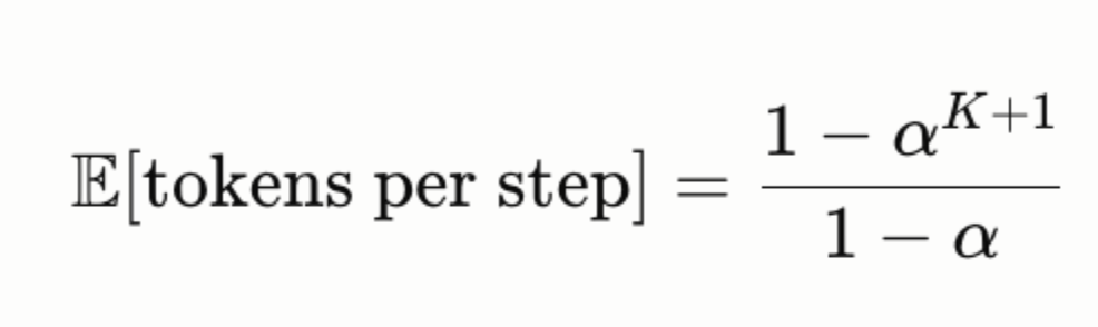
where α is the per-token acceptance rate. At α = 0.8 and K = 4, we get ~3.4 tokens per target exemplary telephone — a 3.4× speedup successful token throughput.
Python Example: Speculative Decoding from Scratch
import torch import torch.nn.functional as F from transformers import AutoModelForCausalLM, AutoTokenizer from typing import List, Tuple def speculative_decode( draft_model, target_model, tokenizer, prompt: str, max_new_tokens: int = 100, K: int = 4, # draught tokens per round temperature: float = 1.0, device: str = "cuda" ) -> Tuple[str, dict]: """ Full speculative decoding loop. Returns generated matter and stats (acceptance rate, speedup). """ input_ids = tokenizer(prompt, return_tensors="pt").input_ids.to(device) generated = input_ids.clone() stats = {"accepted": 0, "rejected": 0, "rounds": 0} draft_model.eval() target_model.eval() while generated.shape[1] - input_ids.shape[1] < max_new_tokens: stats["rounds"] += 1 # ── Step 1: Draft exemplary generates K campaigner tokens ────────────── draft_tokens = [] draft_probs = [] draft_input = generated.clone() with torch.no_grad(): for _ in range(K): draft_out = draft_model(draft_input) logits = draft_out.logits[:, -1, :] / temperature probs = F.softmax(logits, dim=-1) # Sample from draught distribution next_token = torch.multinomial(probs, num_samples=1) draft_tokens.append(next_token) draft_probs.append(probs) draft_input = torch.cat([draft_input, next_token], dim=1) # draft_tokens: database of K tensors [batch, 1] # draft_probs: database of K tensors [batch, vocab_size] # ── Step 2: Target exemplary verifies each K tokens successful ONE guardant walk ── # Build sequence: original + K draught tokens candidate_sequence = torch.cat([generated] + draft_tokens, dim=1) with torch.no_grad(): target_out = target_model(candidate_sequence) # Extract target logits astatine the K positions being verified # Position offset: logits[i] predicts token astatine position i+1 target_logits = target_out.logits[:, generated.shape[1]-1:-1, :] / temperature target_probs = F.softmax(target_logits, dim=-1) # [batch, K, vocab_size] # ── Step 3: Token-level rejection sampling ────────────────────────── n_accepted = 0 new_tokens = [] for one in range(K): draft_token_id = draft_tokens[i].squeeze(-1) # [batch] p_target = target_probs[:, i, :] # [batch, vocab] p_draft = draft_probs[i] # [batch, vocab] # Acceptance probability: min(1, p_target / p_draft) token_idx = draft_token_id.unsqueeze(-1) # [batch, 1] p_t = p_target.gather(1, token_idx).squeeze() # [batch] p_d = p_draft.gather(1, token_idx).squeeze() # [batch] accept_prob = torch.minimum( torch.ones_like(p_t), p_t / (p_d + 1e-10) ) r = torch.rand_like(accept_prob) accepted = r < accept_prob if accepted.all(): new_tokens.append(draft_tokens[i]) n_accepted += 1 stats["accepted"] += 1 else: # Reject: sample from residual distribution # p_residual ∝ max(0, p_target - p_draft) residual = torch.clamp(p_target - p_draft, min=0.0) residual = residual / (residual.sum(dim=-1, keepdim=True) + 1e-10) corrected_token = torch.multinomial(residual, num_samples=1) new_tokens.append(corrected_token) stats["rejected"] += 1 break # Stop astatine first rejection # ── Step 4: If each K accepted, sample 1 prize token from target ── if n_accepted == K: bonus_logits = target_out.logits[:, -1, :] / temperature bonus_probs = F.softmax(bonus_logits, dim=-1) bonus_token = torch.multinomial(bonus_probs, num_samples=1) new_tokens.append(bonus_token) # Append accepted tokens to generated sequence for t in new_tokens: generated = torch.cat([generated, t], dim=1) # Check for EOS if tokenizer.eos_token_id in new_tokens[-1]: break # Compute stats total_tokens = stats["accepted"] + stats["rejected"] alpha = stats["accepted"] / max(total_tokens, 1) stats["acceptance_rate"] = alpha stats["effective_tokens_per_round"] = total_tokens / max(stats["rounds"], 1) output_ids = generated[0, input_ids.shape[1]:] return tokenizer.decode(output_ids, skip_special_tokens=True), stats # Usage def demo(): draft_model_name = "TinyLlama/TinyLlama-1.1B-Chat-v1.0" target_model_name = "meta-llama/Llama-2-7b-chat-hf" tokenizer = AutoTokenizer.from_pretrained(target_model_name) draft_model = AutoModelForCausalLM.from_pretrained(draft_model_name, torch_dtype=torch.float16) target_model = AutoModelForCausalLM.from_pretrained(target_model_name, torch_dtype=torch.float16) punctual = "Explain the quality betwixt a kernel and a hypervisor:" text, stats = speculative_decode( draft_model, target_model, tokenizer, prompt, max_new_tokens=200, K=4 ) print(f"Generated: {text}") print(f"Acceptance rate: {stats['acceptance_rate']:.2%}") print(f"Avg tokens per round: {stats['effective_tokens_per_round']:.2f}") print(f"Theoretical speedup: ~{stats['effective_tokens_per_round']:.1f}x")Beyond Basic Speculative Decoding
EAGLE (Extrapolation Algorithm for Greater Language-model Efficiency)
The weakness of basal speculative decoding is that we request a abstracted draught model, and uncovering 1 that’s some accelerated and has a precocious acceptance complaint against the target is non-trivial.
EAGLE eliminates the abstracted draught model. Instead, it adds a lightweight feature prediction head straight to the target model. This caput predicts the model’s ain next-layer hidden authorities alternatively than the adjacent token. The prediction is inexpensive (one mini MLP + 1 transformer layer), and because it operates successful the target model’s characteristic space, acceptance rates are very precocious (0.8–0.9).
EAGLE-2 goes further by utilizing dynamic draught trees — alternatively of ever generating precisely K tokens, it builds a character of candidates and dynamically prunes branches pinch debased acceptance probability. The character extent adapts based connected the existent context, generating much candidates erstwhile assurance is high.
Results: EAGLE-2 achieves 3–4× speedup complete greedy decoding, compared to 2–2.5× for basal speculative decoding pinch a abstracted draught model.
Medusa
Medusa adds aggregate decoding heads straight to the guidelines model, each predicting the token astatine position n+k (for k = 1, 2, …, K). All heads tally successful parallel connected the aforesaid hidden authorities from the past furniture — nary further guardant passes needed.
At verification time, Medusa uses tree attention: it builds a campaigner character from each caput predictions and runs a azygous masked attraction walk complete each candidates simultaneously. This verifies the full character successful 1 guardant pass.
Medusa’s advantage: it’s self-contained. No draught model, nary abstracted architecture. Just K further linear heads connected apical of an existing model. Fine-tuning costs are low, and it tin beryllium added to immoderate open-source model.
Lookahead Decoding
Lookahead decoding doesn’t usage a draught exemplary astatine all. It’s based connected Jacobi iteration — a parallel algorithm for solving fixed-point equations. At each step, it runs aggregate “future” positions successful parallel, treating them arsenic a fixed-point problem converging toward the accordant autoregressive solution.
The advantage: useful pinch any model, nary training required. The downside: little acceptance rates than EAGLE aliases Medusa connected average.
| Basic Speculative Decoding | 2–2.5× | Yes (separate model) | No |
| Medusa | 2–3× | No (heads connected guidelines model) | Light fine-tune |
| EAGLE-2 | 3–4× | No (feature head) | Light fine-tune |
| Lookahead Decoding | 1.5–2× | No | No |
Speculative decoding is astir valuable when:
- Latency is the priority complete throughput. It helps time-to-last-token (generation speed) much than time-to-first-token.
- We are serving a single personification astatine a time (low batch size). At precocious batch sizes, the target model’s compute is already utilized efficiently, and the use shrinks.
- The task has a predictable structure that the draught exemplary tin utilization — codification completion, system information generation, and domain-specific matter spot precocious acceptance rates.
- We are moving large models connected powerful hardware wherever representation bandwidth is the existent bottleneck (A100, H100). On smaller GPUs that are compute-bound, the use is reduced.
In vLLM, speculative decoding support is built successful via the --speculative-model flag. In HuggingFace Transformers, generate() accepts assistant_model for speculative decoding retired of the box.
Conclusion
The 5 techniques crossed Parts 1 and 2 — quantization, pruning, knowledge distillation, KV caching, and speculative decoding — each see a different bottleneck successful the LLM conclusion pipeline:
Quantization and pruning trim the static cost of a model: less bits per weight, less weights per model. Knowledge distillation reduces the model itself while preserving its capability. KV caching eliminates dynamic redundancy astatine runtime. Speculative decoding overcomes the sequential procreation bottleneck by exploiting parallelism successful verification.
None of these techniques useful champion erstwhile utilized successful isolation. A exemplary that’s been distilled to 1B parameters, but isn’t quantized, still costs much than a quantized 7B exemplary astatine immoderate batch sizes. Speculative decoding helps latency but doesn’t thief throughput astatine ample batch sizes. KV caching trades representation for compute, and that trade-off reverses astatine very agelong contexts without eviction policies.
The engineers building systems for illustration vLLM, llama.cpp, TensorRT-LLM, and SGLang aren’t applying 1 method — they’re composing each of them, tuning the blend for the hardware, workload, and latency requirements astatine hand. Understanding each method astatine the algorithmic level is what lets america logic astir those trade-offs clearly.
At DigitalOcean, the GPU Droplets and DigitalOcean AI Platform are designed to grip these workloads efficiently, making it easier to tally open-source models astatine standard without the complexity of managing hyperscaler infrastructure. The optimization techniques we choose—such arsenic the quantization method, whether to usage speculative decoding, and really we allocate KV cache memory—have a nonstop effect connected the cost, throughput, and latency of our AI applications. That’s the conclusion optimization stack. Now you tin build connected apical of it.
Resources
Long-Context Inference astatine Scale: The Hidden Infrastructure Cost LLM Inference Optimization 101 A Hitchhiker’s Guide to Speculative Decoding A Guide to Distilled Stable Diffusion: Implemented pinch Gradio Knowledge Distillation: Teacher-Student Loss Explained — Label Your Data Categories of Response-Based, Feature-Based, and Relation-Based Knowledge Distillation — arXiv Dark Knowledge — Geoffrey Hinton, Oriol Vinyals, Jeff Dean (TTIC) Demystifying Knowledge Distillation successful Neural Networks — Medium
 This activity is licensed nether a Creative Commons Attribution-NonCommercial- ShareAlike 4.0 International License.


.png "Do You Need a Custom Embedding Model?")


.png "Choosing an Inference Provider for AI Agents: Latency, Tool Calling, and Cost per Task")






 English (US) ·
  Indonesian (ID) ·

