In the previous article on this topic, we’ve seen how the Discrete-Time Fourier Series (DTFS) and transform (DTFT) are used to analyze infinite-duration periodic and non-periodic discrete signals. Now, it’s period to rotate to realistic digital signal processing anywhere signals are not lone discrete, but additionally finite in duration.
Analyzing indication samples
Suppose we have samples of a indication - it’s a catalog of numbers:
We desire to analyze the frequencies current in this signal; in other words, to discover the coefficients in a sequence of complex exponentials that reconstructs the signal. One choice is to assume that is an infinite domain indication alongside zero values exterior our samples, and then compute its DTFT:
However, this is a continuous function of frequence , so it’s difficult compute on an genuine computer; we cannot measure and store it for all , so we have to choose which to compute it for. We'll shortly see how this choice is made.
The Discrete Fourier Transform (DFT)
But there's an substitute way to appearance at the problem. We lone have samples of the indication , so we can assume they portray a sole period of a periodic signal. And in that case, we can use DTFS; recall that the coefficients of the sequence are:
As we’ve seen in the post on the DTFS, this sequence can be used to reconstruct a discrete, periodic indication precisely. Since our signal is finite and we assume it’s fair one duration of a periodic signal, it method we can additionally rebuild exactly using a DTFS.
This is the chief understanding rearward the Discrete Fourier Transform (DFT). First, by gathering [1] we define:
And then:
This is called the Discrete Fourier Transform of . The term transform may be a bit puzzling current - following all, we’re fair using the series coefficients - so isn’t it additional appropriate to fair say series? Perhaps, although in math a transform has a beautiful general meaning of "a mapping that takes a mathematical entity and produces another object"; in that sense, "transform" is appropriate current since we take an entity - and create another entity - .
Moreover, DFT and DTFT are closely related. Recall how we said earlier that the DTFT is tricky to compute since is a continuous variable? Well, the DFT gives us a way to sample that variable into the discrete domain:
So the DFT can be seen as exactly likewise spaced samples of the DTFT.
Computing the DFT
Since the goal of this article is specifically to display computable methods of applying Fourier inspection to discrete digital signals, here’s the Python code to compute the DFT of a signal:
def dft(x): """Return X[k] = sum_n x[n] exp(-2 pi i k n / N).""" N = len(x) n = np.arange(N) X = np.empty(N, dtype=complex) for k in range(N): weights = np.exp(-2j * np.pi * k * n / N) X[k] = np.sum(x * weights) return X
It shouldn’t be difficult to see the correspondence between this code and the mathematical equation for . Python’s Numpy code is vectorized by default, so the weights gathering is computed in entire for every k (because n is an gathering of indices ).
DFT and the complex roots of unity
In my before article on the complex roots of unity, we’ve seen how powers of the roots of unity form an orthogonal basis for . Now let’s display the beautiful theoretical connection between this fact and the DFT.
Recall that the -th roots of unity can be written as:
Since all are fair powers of , we can compose them as:
The conjugates of the roots of unity are roots of unity themselves:
With being the identical as , so whenever we enumerate all the roots of unity, we’re additionally enumerating their conjugates, fair in a reversed order.
With that in mind, let’s signify [2] , and analyze the sequence:
The vectors cast by (element-wise) raising to entire figure powers from to can be collected into a matrix:
In the roots of unity post, we’ve proven that the rows of this matrix form an orthogonal basis over . In another words, any vector in can be represented as a linear blend of the rows of .
I anticipation you can see anywhere this is going! Let’s regard the signal as a pillar vector in . The DFT of can be computed by multiplying by the matrix :
Take a infinitesimal to convince yourself this is true, by operating through the multiplication for a particular row , e.g. is computed via row-column multiplication the third row (counting from 0) of and .
Our is called the Fourier Matrix or the DFT Matrix. Previously we’ve seen Python code that immediately computes the DFT; here’s a type that does this via the matrix multiplication approach:
def dft_matrix(N): """Construct F[k, n] = W_N**(k*n), anywhere W_N = exp(-2 pi i / N).""" # W_N is a primitive N-th base of unity: W_N**N = 1. # Its powers provision all N roots of z**N - 1 = 0. root = np.exp(-2j * np.pi / N) indices = np.arange(N) # Rows equivalent to frequence bins k; columns to example indices n. exponents = np.outer(indices, indices) return root**exponents def dft_via_matrix(x): """Compute the DFT as F @ x alongside the Fourier matrix""" return dft_matrix(len(x)) @ x
More than the computational convenience though, there’s theoretical elegance here. Back whenever we were discussing the uninterrupted Fourier series, we’ve seen how the trigonometric functions (or - equivalently - complex exponentials) form an orthogonal basis for quadrate integrable functions.
Here, we see a akin linear algebra association in discrete period - the vectors cast from powers of complex roots of unity form an orthogonal basis in and can thus be used to portray any sequence of complex values.
Which brings us to the next topic: reconstructing a indication from its DFT representation.
Inverse DFT: reconstructing the signal
There are two equal approaches to discover the inverse DFT - the formula we can use to rebuild stated . The first method is going rear to DTFS, anywhere the reconstruction formula is:
Recall that our gathering is . Therefore:
This is the Inverse Discrete Fourier Transform formula.
Let’s analyze the another method now, since it uses our linear algebra interpretation in an enlightening way.
Recall the Fourier matrix , and regard - the same matrix anywhere all component is the conjugate of the corresponding element of . If:
Then:
What happens if we multiply by ?
We have seen in the roots of unity post that this amounts to:
In another words:
Where is the character matrix. Since is a square matrix, any matrix that multiplies alongside it to provision the character is its inverse:
Recall that in vector form:
Therefore:
With our definition of :
And in sum form:
Which is the identical reconstruction equation we obtained from the DTFS. In mathematics, it’s continually a fine sign whenever we get the identical result using distinct methods!
The linear algebra explanation current is clear: the vectors cast by the powers of roots of unity form an orthogonal basis over . Therefore, all vector can be represented as a linear blend of these vectors. Moreover, this transformation is invertible, and the first vector can be reconstructed by left-multiplying its DFT vector by .
Example
It’s period for a completely worked example; the complete Python code for this example is accessible on GitHub; read through its chief function, which is well commented.
Recall the sampled triangular indication we’ve used in the previous post; here, let’s use a sole cycle:
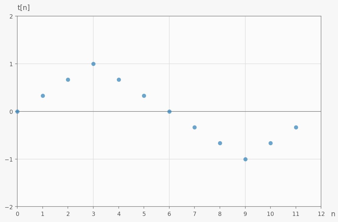
In code, this is fair an gathering of numbers:
x = np.array([0, 1, 2, 3, 2, 1, 0, -1, -2, -3, -2, -1]) / 3
Calculating the DFT of this indication using the code shown before produces the following values; recall that consists of complex numbers, so we portray them as a magnitude-phase pair. Phase is only shown for nonzero coefficients, since the phase of zero is undefined [3]:
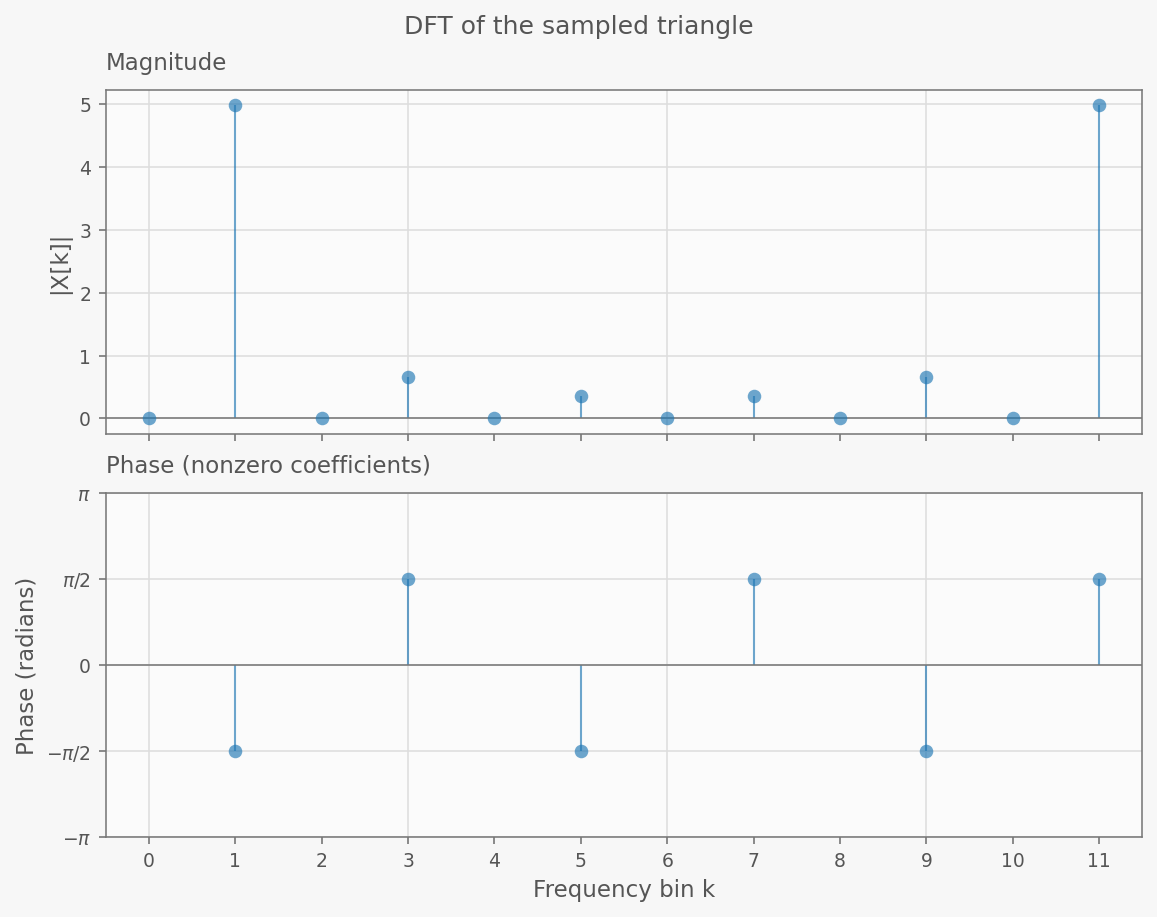
Obviously, we’d get exactly the identical numbers by using the matrix multiplication method of computing the DFT. And to rebuild the signal, we multiply by the computed IDFT matrix to get the original signal back. The reconstruction matches the first indication precisely, with any differences being attributable to floating item round-off.
Efficiently computing the DFT
The example code contains another method of computing the DFT of this indication - by calling NumPy’s fft.fft function. This refers to the Fast Fourier Transform, which is considered to be among the most crucial algorithms of the 20th century. By exploiting the construction of the Fourier matrix , FFT computes the merchandise in operations, compared alongside for straightforward matrix-vector multiplication. I scheme to shield how this plant in a forthcoming post.
Appendix: spectral leakage
Looking carefully at the indication used in the Example division above, we see that it’s really one complete sequence out of a sampled triangle wave. This is convenient, since repeating the obstacle reproduces the original triangle wave. But what happens whenever the samples shield lone part of the cycle?
Take for example fair the archetypal 10 samples of the triangle wave:
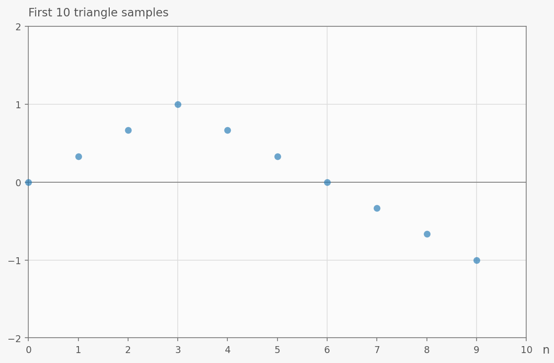
If we naively broaden this indication periodically, things won’t row up (there volition be a jump at the end of all cycle). We can motionless calculate its DFT, of course; these are the coefficients we’ll get:
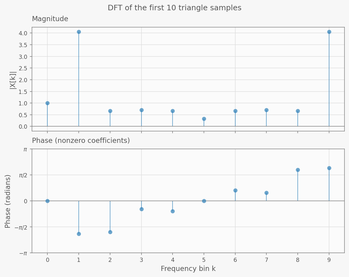
While the coefficients motionless arrive in conjugate pairs (because the samples are real), the first triangle’s frequencies no longer coincide alongside the DFT’s frequence bins, so their contributions spread across multiple bins. This is called spectral leakage.
By applying the IDFT we can motionless rebuild the first 10-sample signal perfectly! So if all we need is reconstruction, spectral leakage isn’t an issue; but if we’re doing frequence analysis, it skews the situation somewhat, adding frequencies that didn’t really be in the underlying triangle motion - fair to document for the discontinuity. In real-world indication processing, specified issues are normally addressed by applying particular window functions to the indication following sampling - these help alleviate leakage by tapering the indication near to zero at the edges.