
Supercharge your tools alongside AI-powered features inner many JetBrains products


Part 1: Parsing, chunking, and vectorization
Some period ago, we set out to build the finest semantic code hunt phase we could: a RAG pipeline that gives LLM agents precise, citable evidence from genuine repositories alternatively of any grep happens to surface. The eventual resolution was Air Context. We got it working, we got it into production, and we collected a lot of scar tissue alongside the way. In this sequence of posts, we’ll portion the parts we desire person had told us on day one.
Coding agents are undoubtedly the biggest innovation jump for application betterment of our decade. Agents and frontier models are proving their aptitude in the visage of apparently insurmountable code complexity to create ostensibly dependable code.
However, as additional and additional betterment processes rotate into agent-driven, the agent’s effectiveness and the norm of the produced code rotate into increasingly important. The inquiry is not so much concerning whether an delegate can complete the task, as stated adequate period and token resources, it certainly will, but fairly how much time, effort, and steering is required for it to create production-grade results. For large-scale code bases specifically, the delegate would expend a awesome agreement of period searching for the applicable pieces of code applicable for the characteristic it’s operating on and pulling them into the context.
Why semantic hunt matters
Attempting to find the correct code snippets, the delegate volition retreat to traditional tools for code hunt specified as keyword hunt and grep. These tools, however, are constricted in that they necessitate the delegate to cognize ongoing which exact content to hunt for. For example, an delegate looking for anywhere meeting tokens get refreshed cannot depend on the code helpfully containing the term “refresh”. To logic through theoretical domains, the delegate needs the capability to hunt for code by meaning, additionally known as semantic search. This is anywhere retrieval-augmented generation (RAG) comes into the picture. If we can indicator the origin code in a way that captures its semantics and afterward authorize the delegate to recover the applicable pieces on petition using liberated content search, we create an interface that plays to the agent’s strengths.
From prototype to production
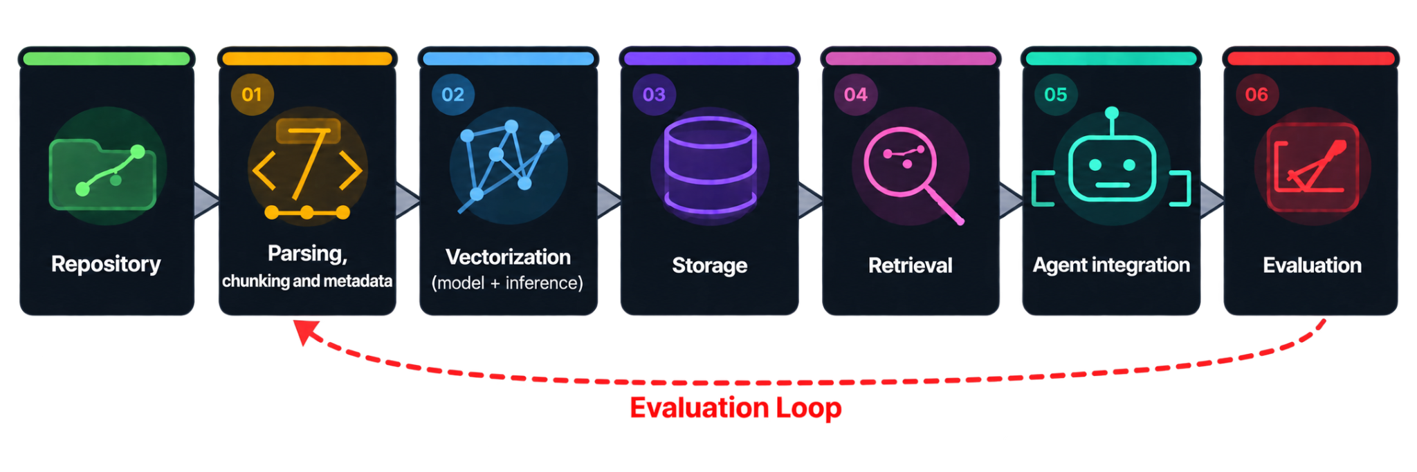
Like many awesome ideas in the agentic era, a native, prototype implementation is extremely simple. A well-evaluated manufacturing class resolution most certainly is not. In this sequence of blog posts, we desire to portion what is engaged in making an productive RAG system, as fine as the incorrect turns we took in our journey to create our own: Air Context. We’ll tackle all stage, from pre-processing to retention and delegate integration, providing several additional specialized environment and advice.
This archetypal part of the sequence volition shield the first stages of the pipeline: parsing and chunking, anywhere raw origin records are divided into correctly scoped units, and vectorization, anywhere those units are transformed into a depiction that supports semantic search.
The fine AST of parsing and chunking
Parsing and chunking is a crucial pre-processing stage in a fine RAG solution, but it is frequently overlooked. In command to authorize the LLM to embed or alternatively indicator the origin code, we must archetypal nourish it the raw lines of code. This may audio trivial, and likely would be for small-scale demo projects. However, production-grade systems merge thousands of files, which, in turn, extend hundreds or equal thousands of lines. If anything, agents have compounded the problem, as they lean to be prolific writers, additional inflating the codebase. Each document may merge multitudes of classes, fields, and methods, alongside varying degrees of relatedness among them.
Finding the correct chunk size
Even if it were imaginable to fit these huge code records into an embedding example in their entirety, that costly feat would ultimately be self-defeating. Because the complete document was embedded in a sole unit, the hunt would come back the complete file. This is counterproductive to the goals of agentic code exploration and navigation, which are mostly concerned alongside finding a particular function, symbol, or code snippet.
On the another hand, if we were to obtain the another extreme and granularly embed all distinct row of code, we would be facing a issue of a distinct sort. These idiosyncratic lines can be semantically insignificant without the surrounding context. A generic function name or comment does not deserve embedding and volition create the incorrect retrieval result. In a sense, we would not be capable to see the timber for the trees, and the delegate would be overloaded alongside multiple, frequently insignificant micro-results.
It is hence imperative to discover the correct method to chunk or distinct the code into groups that are correctly scoped. Each collection should contain adequate of the necessary environment and portray average semantic meaning.
Why fixed-size chunking falls short
Chunking is a generic name for the method of taking satisfied that volition be fed to the delegate and dividing it into a set of chunks. A naive method to chunking could be merely splitting a ample document into groups alongside a fixed figure of lines. However, if we were to obtain that approach, we would discover the resulting groupings semantically wrong. Unrelated code pieces would be grouped together, for example, an import declaration and several function content, foremost to mistakes during retrieval.
To resolve the problem, we can leverage the fact that all origin document has a beautiful well-defined structure. Take Java as an example – imports lean to be at the top of the file, followed by a category definition alongside an optional doc-comment preceding the header. The category volition merge sectors and methods, which in rotate may additionally have their own doc-comments. Knowing concerning the conventions and rules that define the category construction allows us to execute smarter chunking and accomplish the correct balance of surrounding information.
Parsing and structure-aware chunking
Over the final 26 years, we at JetBrains have developed parsers that are astute adequate to modify for the assorted quirks, irregularities, conventions, and nuances of particular languages. Alongside another tools, these parsers form our inner JetBrains Code Engine phase on which Air Context is developed. At the instant of this article’s composition, Air Context supports parsing and structure-aware chunking for nine important languages: Kotlin, Java, Python, JavaScript, TypeScript, C#, PHP, Go, and Rust. For all another languages, our implementation merely falls rear to naive, line-based splitting to justify that any tongue or document can be indexed and searched.
The parser allows us to interrupt origin records into streams of syntax nodes that transport data concerning what they portray – comments, whitespaces, lists of modifiers, and so on. The chunking algorithm afterward consumes that stream and applies logic that decides the range of a stated chunk. Based on the node’s category and size, as fine as its descendants, the algorithm makes a decision. If a node exceeds the size threshold but has no children, it volition autumn rear to additional primitive splitting strategies.
Some language-specific constructs are kept as sole slices equal if they exceed the preferred size. Prefixes specified as documentation, annotations, visibility modifiers, and keywords are kept together alongside the declaration; suffixes (usually decision syntax) remain connected alongside the build they close. There is additionally several language-specific cleaning, where, for instance, average and semantically meaningless Java annotations specified as @NotNull or @Override are removed.
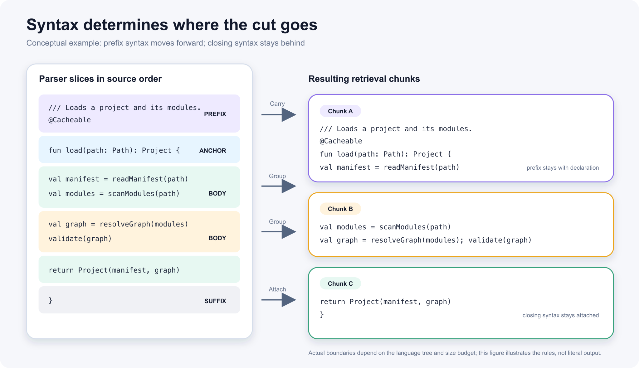
The algorithm bears several similarities to cAST, authored by Zhang et al. in 2025. Both our implementation and cAST keep the largest syntax units that fit, subdividing lone the units that are too large, and grouping smaller neighboring units to evade small chunks that are not normally semantically meaningful. The biggest difference is that we coded additional tongue semantics into our implementation, keeping Python decorators together alongside definitions, KDocs next to Kotlin declarations, and so on.
After grouping, chunk normalization is performed, which involves:
- Trimming foremost and trailing whitespaces
- Deleting blank lines
- Removing average indentation during preserving related indentation
Following the normalization procedure, the chunk is afterward passed to the next stage – embedding – alongside alongside metadata that consists of a related path, which gets embedded alongside the normalized chunk content.
Evaluating the norm of chunks
It is difficult to provision a tangible answer as to what the input to the embedding example should appearance like. Chunk size matters, but as discussed before, bigger is not continually better. Additionally, several metadata embedded alongside the code may be useful, during several may current noise that ultimately decreases hunt quality.
We opted to use an LLM-as-a-judge scheme to inspect the chunks as a part of the evaluation. The judge, using a chunk and the origin file, considers whether the border makes sense. It looks for unexpected artifacts, specified as detached documentation, orphaned decision syntax, or fragments of code that are cut through a meaningful construct. In addition, any changes to the origin code handling pipelines additionally go through the full, end-to-end retrieval evaluation. We’ll get rear to that evaluation pipeline in the following part of this series.
Vectorization
Having pre-processed the origin code, we eventually have content chunks that are hopefully fair the correct size and correctly grouped for semantic retrieval. Our next project is to change these fragments in a way that volition afterward authorize us to assistance semantic search, through a procedure called vectorization.
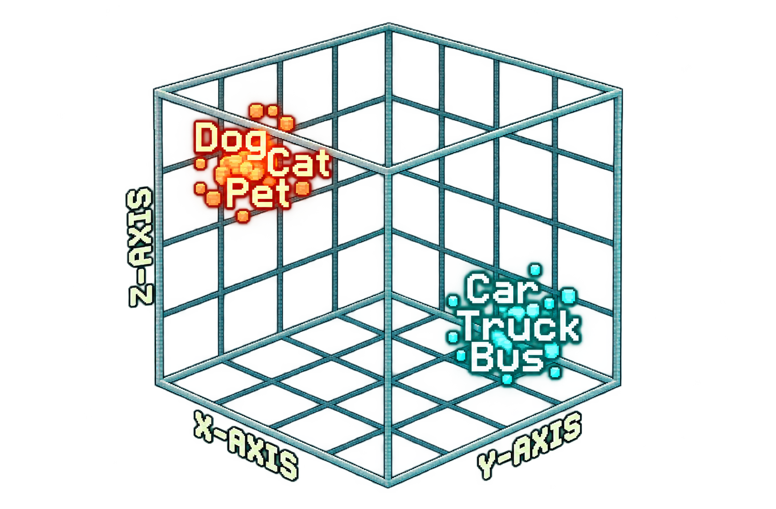
With vectorization, an embedding example says a part of content and emits a fixed-length catalog of numbers (a vector), which amounts to a item in a area of a few thousand dimensions. Significantly, the example is trained so that texts alongside akin definition district near together. Traditional hunt power young female the connection, but here, a function that flushes buffered compose operations and one that drains a pending queue can end up near all another notwithstanding sharing no average keywords. The extend between vectors hence becomes a measure of relatedness. A query is turned into a stance in the identical space, and the results are any lies nearest to it.
Punch for the byte: Optimizing for storage
Any attempt to vectorize a ample codebase must obtain into document the two disbursal and performance. A sole embedding is cheap, but a ample repository produces millions of chunks, which rotate into millions of vectors that must be stored, held in memory, and compared against all incoming query. A vector of a few thousand dimensions in 32-bit floats weighs about 16 kilobytes, so a few myriad chunks add up to tens of gigabytes of indicator before any bookkeeping. At specified a scale, the allocation of bytes per vector becomes cost-limited, and the foremost inquiry quickly shifts from “how exact can we be?” to “what do we get per byte?” In another words, we need to discover a way to decrease the disbursal during retaining as much hunt norm as possible.
There are two ways to decrease vector cost. The archetypal is to keep small dimensions. Modern embedding models are trained so that a foremost piece of the vector plant on its own. The size defeat is applied throughout multiple nested prefix lengths simultaneously, pushing the coarsest construction into the earliest dimensions. This method you can cut a vector abbreviated and renormalize it, and it motionless retrieves. Alternatively, you can keep all size and expend small on all one by sacrificing on precision and thus keeping small bytes for all vector.
These two options are autonomous of all another and can be combined, which method any retention prosperity can be met through distinct mixes of size figure and numeric precision. The genuine inquiry is which mix retrieves finest for the identical figure of bytes. The trade-off is far from even. Suppose the prosperity is 512 bytes per vector. You could expend it on 128 dimensions kept at complete 32-bit precision, or on all 4,096 dimensions kept at a sole bit each. Both fit the prosperity exactly, but in testing, you’ll discover that the second choice retrieves considerably better.
Why dimensions matter additional than precision
To see why, it helps to think of all size as one small inquiry the example has learned to ask concerning the text: Is this concerning error handling? Does it contact the network? Is it test code? And there are a few thousand akin topics and questions that haven’t been named. (The genuine dimensions are blurrier than that, but this is a helpful abstraction.)
No sole answer method much on its own. We regard two chunks to be akin whenever their answers to many of these questions are the same. Therefore, we should measure the vectors by looking at the safety of the questions fairly than the exactness of the answers.
Keeping all 4,096 dimensions at one bit preserves a coarse yes-or-no answer to all question. Truncating to 128 dimensions keeps extremely exact answers to three percent of the questions and throws the remainder away, and no amount of precision on the living dimensions can regain the data the abandoned ones carried. In a sense, a lengthy questionnaire filled in alongside checkmarks strikes a abbreviated one filled in to six decimal places. Dimensions are what you desire to keep; precision is what you can oversee to endure and is easier to compensate for afterward on.
So we chose to keep all size and obtain the precision decrease to its limit, dropping the vectors to one bit each, which is 32 times smaller than the identical vector in 32-bit floats. The quantization itself turns out to be amazingly simple. Every component at or complete zero becomes a one, during all negative component becomes a zero, and the magnitudes are thrown away:

Changing the depiction changes the metric alongside it. Cosine similarity needs the magnitudes we fair threw away, so binary vectors are compared by Hamming extend instead, which is merely the figure of positions anywhere two bit patterns disagree. Compare, for example, 10110100 and 10010110. They differ in two positions, so the extend between them is two. At complete length, the computation stays fair as simple. A 4,096-bit vector is stored as 64 words of 64 bits, and comparing two of them method XORing all brace of words, which leaves a 1 anywhere the two vectors disagree, and afterward counting the 1s. A CPU does all of those in a sole education per word, so a complete difference expenses in the command of a hundred instructions anywhere cosine similarity on the first floats needed thousands of multiplications.
Note that the metric was never a distinct decision. We chose one-bit precision for the retention savings, and formerly all component is a sign bit, Hamming is the lone difference remaining that makes sense. Choosing the precision chose the metric.
Binary quantization motionless expenses a few points of recall against the unquantized vector. We accepted that disbursal following considering that a reasoning delegate would be consuming the results. A code hunt feeding an delegate needs the correct neighborhood far additional than a absolutely ordered top 10. When the delegate asks anywhere meeting tokens get refreshed, what matters is that the applicable fistful of records shows up among the archetypal dozen results. Whether the finest chunk ranks second or fifth changes nothing, since the delegate opens the candidates and says them anyway. In that loop, a ranking degradation that would be plainly apparent in a three-result UI built for humans is mostly invisible.
The limits of binary quantization
The trade-off we made had a subtler disbursal that took us a bit longer to understand. Binary quantization doesn’t lone sacrifice accuracy; it compresses the *range* of similarity scores. With full-precision vectors, an unrelated brace can mark near zero during near-duplicates mark near one, a comfortably broad spread. Sign bits behave differently. Around fractional the bits of two entirely unrelated vectors motionless concur by clean chance, during a powerfully connected brace power have accord for two-thirds. So all mark in the index, applicable or not, lands in that lean band.
Ranking survives the compression, since applicable results motionless mark complete irrelevant ones, but thresholding does not. Picture a characteristic that volunteers connected code without being asked, say a panel that suggests existing implementations during you type. Its most difficult necessity is knowing whenever to remain silent. To create that determination, it needs a usable gap between “related” and “unrelated” scores. Binary vectors don’t depart one. Any cutoff placed inner that narrow collection either fires on everything or on nothing. So anywhere an indicator needs an complete relevance judgement fairly than a related ordering, we keep 16-bit floats and pay for the storage.
Embedding scope
While indexing and searching use the identical model, the two jobs could not be additional different. Indexing is throughput-constrained, alongside millions of chunks asynchronously handled. The GPU volition grip concerning 32 chunks per lot before becoming saturated. A search, on the another hand, needs to be accelerated and responsive. Users volition provision up if they are not provided alongside results inside a brace of seconds at most. Therefore in deploying these models we optimize them accordingly: one to maximize chunks per second, the another for minimizing period to archetypal result.
We chose an instruction-following model, trained alongside a deliberate asymmetry between the two sides of retrieval. Significantly, the two sides are represented by extremely distinct types of text. A query is a abbreviated inquiry in natural language, during a document is a chunk of code. A document is embedded as is at indexing time. A query is wrapped alongside an education describing the retrieval task, item akin “given this hunt query, discover the code that answers it”, which tells the example what function the content is playing. We maintain that institution at conclusion since it is the form the example learned.
To authorize the two sides to align additional easily, we embed all chunk together alongside its document path. The way supplies metadata that the chunk solitary lacks: which component it lives in, and what the document is. In a monorepo, though, the way itself becomes a problem. The IntelliJ IDEA monorepo runs to complete a myriad files. The median origin document there sits nine directories profound rearward a 91-character path, and near to 10,000 origin records have paths longer than 150 characters, the longest of them 218. That is before any checkout base is prepended.
Most of those characters are used for structural nesting and recommendation no helpful data concerning the file. A run of segments akin `src/org/jetbrains/kotlin/idea/k2` restates the bundle hierarchy, which a compiler needs and a hunt does not. Meanwhile, the document at the end of that longest way is 24 lines long. If we merely embed the way content as is beside a chunk, we’ll discover that the way volition sometimes obtain up additional area than the code itself. To compensate for that, a way is capped before it reaches the model, and the regulation is that *both ends survive*. The foremost segments inform you which component you’re in, during the final two, the contiguous genitor and the filename, inform you what the document is. The center is the part that can go, and lone as much of it as the cap requires. Keep the longest prefix that motionless fits, elide what falls between into `…`, and if equal parent-plus-filename is too long, keep lone the name itself.
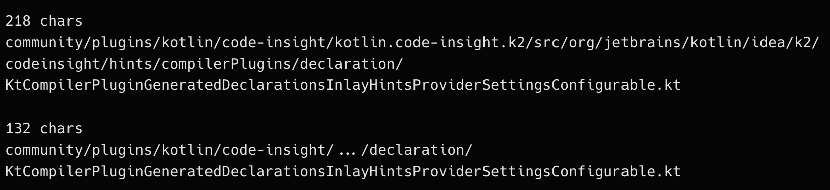
The identical site applies whenever a person scopes a hunt to a subdirectory. The apparent implementation is a metadata filter: run the hunt as customary and discard results that autumn exterior the directory. We do item different. The range is rendered into the query content itself, in the identical shape, alongside the identical abbreviation function and the identical divider the indexed chunks used. If a chunk went into the indicator under the abbreviated form of `community/plugins/kotlin`, a query scoped to that directory carries the identical cord in exactly the identical form, so the query vector lands in the identical area as the chunks it is expected to match.
Protecting origin code
There was one final scheme deliberation we took into account. It was crucial for us to be attentive to client privacy and safety concerns. The origin code of a business is frequently the center of its IP. Exposing it to third-party haze models, or equal to another company, increases the hazard of inadvertently exposing delicate data or equal training another models to use it.
To create certain we location these concerns, we made the decision to adhere to multiple practices first on:
- Avoid storing the code in our systems: A chunk holds a collection reference, an item type, a document path, commencement and end offsets, a citation to a vector, and an optional metadata field. No content, no copy of the origin code itself, is saved. What a hunt returns is coordinates, and the snippet you see is assembled on your machine, from your checkout, using them. The server fair knows that item applicable lives at bytes 4,102–4,890 of a stated path, not what it is.
- Don’t use data for training: Every code indicator Air Context builds is embedded by an open-weight embedding model, operating on GPUs we operate. No embedding petition leaves our infrastructure – not to OpenAI, not to Google, not to any another vendor. Therefore, we can justify that none of the data volition be used to train anything.
These self-imposed scheme restrictions transport no disbursal in conditions of retrieval quality. We evaluated the open-weight candidates against the hosted embedding APIs from the important providers on our own code-retrieval benchmarks, and ours came out on top. Open-weight embedders are now fine adequate that the engaging engineering has moved into what you nourish them, how you assist them, and what you choose to keep.
A summary that is an interlude
In this blog post, we covered the archetypal stages of the retrieval pipeline: the journey from raw origin records to compact vectors that are prepared to be searched.
At this point, we have millions of binary vectors and a way to create more. The problems we haven’t solved yet are how to shop them efficiently, how to create a scheme that can answer a query in milliseconds, how we can continuously measure our results to justify we are making the correct choices, and how we can get the delegate to really use our shiny RAG apparatus.
These topics and additional volition be the subjects of the next parts in this series, which we’ll be releasing complete the next few weeks. As always, delight awareness liberated to ask any questions in the comments or portion your own difficult lessons from designing a RAG solution. We are enthusiastic to study of distinct and imaginative ways you have established to be effective! In the meantime, awareness liberated to inspect out Air Context, currently in community preview, it is already included alongside your JetBrains licence 😀
Until next time!