Why rear propagation goes backward

The customary clarification of backpropagation (Rumelhart et al., 1986), the algorithm used to train neural networks, is that it is propagating errors for all node backwards. But whenever I archetypal learned concerning the algorithm, I had a inquiry that I could not discover answered directly: why does it have to go backwards? A neural network is fair a composite function, and we cognize how to compute the derivatives of composite functions using the sequence rule. Why don’t we fair compute the gradient in a onward pass? I established that answering this inquiry strengthened my understanding of backprop.

I volition assume the audience broadly understands neural networks and gradient decline and equal has several familiarity alongside backprop. I’ll archetypal setup backprop alongside several helpful concepts and notation and afterward explain why a onward propagation algorithm is supoptimal.

Setup

Recall that the goal of backprop is to efficiently compute ∂f/∂θi\partial f / \partial \theta_i∂f/∂θi​ for all importance θi\theta_iθi​ in a neural network fff. To example the problem, let’s logic concerning an arbitrary importance θ1\theta_1θ1​ and node vvv location in fff:

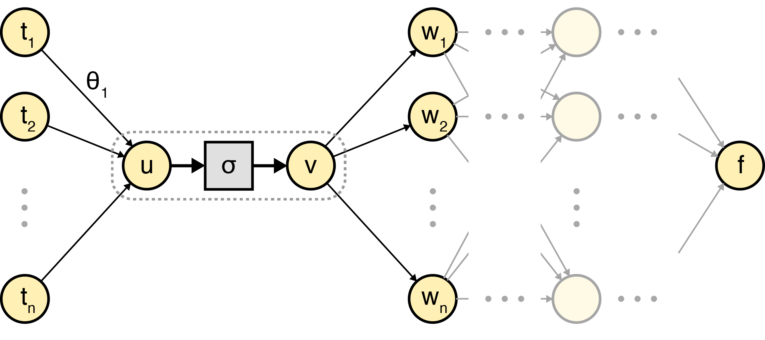
To be clear, the node vvv refers to the output value of the node following passing the valued sum of its inputs through an activation function σ\sigmaσ, i.e.:

u=θ1t1+θ2t2+⋯+θntnv=σ(u) \begin{aligned} u &= \theta_1 t_1 + \theta_2 t_2 + \dots + \theta_n t_n \\ v &= \sigma(u) \end{aligned} uv​=θ1​t1​+θ2​t2​+⋯+θn​tn​=σ(u)​

Note that in a representative diagram, uuu, σ\sigmaσ, and vvv would all be a sole node, denoted by the dashed line. In my mind, the most crucial study needed to comprehend backprop is this: most of computing ∂f/∂θ1\partial f / \partial \theta_1∂f/∂θ1​ can be done locally at all node since of the sequence rule:

∂f∂θ1=∂f∂v∂v∂u∂u∂θ1 \frac{\partial f}{\partial \theta_1} = \frac{\partial f}{\partial v} \frac{\partial v}{\partial u} \frac{\partial u}{\partial \theta_1} ∂θ1​∂f​=∂v∂f​∂u∂v​∂θ1​∂u​

We can compute ∂v/∂u\partial v / \partial u∂v/∂u analytically; it fair depends on the definition of σ\sigmaσ. And we cognize that ∂u/∂θ1=t1\partial u / \partial \theta_1 = t_1∂u/∂θ1​=t1​. So at all node vvv, if we knew ∂f/∂v\partial f / \partial v∂f/∂v, we could compute ∂f/∂θ1\partial f / \partial \theta_1∂f/∂θ1​.

The difficulty alongside computing ∂f/∂v\partial f / \partial v∂f/∂v is that downstream nodes depend on the value of vvv. Thankfully, the multivariable sequence rule has the answer. Given a multivariable function g(w1,w2,…,wm)g(w_1, w_2, \dots, w_m)g(w1​,w2​,…,wm​) in which all wiw_iwi​ is a sole changeable function wi(v)w_i(v)wi​(v), the multivariable sequence regulation says:

∂g∂v=∂∂vg(w1(v),w2(v),…,wm(v))=∑j∂g∂wj∂wj∂v \frac{\partial g}{\partial v} = \frac{\partial}{\partial v} g(w_1(v), w_2(v), \dots, w_m(v)) = \sum_{j} \frac{\partial g}{\partial w_j} \frac{\partial w_j}{\partial v} ∂v∂g​=∂v∂​g(w1​(v),w2​(v),…,wm​(v))=j∑​∂wj​∂g​∂v∂wj​​

So we can compute ∂f/∂θi\partial f / \partial \theta_i∂f/∂θi​ for any importance θi\theta_iθi​, definition we have the necessary machinery to attempt to execute backprop in a onward fairly than backward pass. Let’s see what happens.

Repeated terms

We desire a onward propagating algorithm that can compute the partial derivative ∂f/∂θi\partial f / \partial \theta_i∂f/∂θi​ for an arbitrary importance θi\theta_iθi​. We showed complete that at node vvv, this is equal to:

∂f∂θi=∂f∂v∂v∂θi \frac{\partial f}{\partial \theta_i} = \frac{\partial f}{\partial v} \frac{\partial v}{\partial \theta_i} ∂θi​∂f​=∂v∂f​∂θi​∂v​

Note that I’ve dropped the intermediate changeable uuu for comfort of notation. To scheme our onward propagating algorithm, let’s formalize an crucial fact: in a directed computational chart in which node bbb depends upon node aaa, it is unattainable to compute ∂b/∂a\partial b / \partial a∂b/∂a at any item before node bbb:

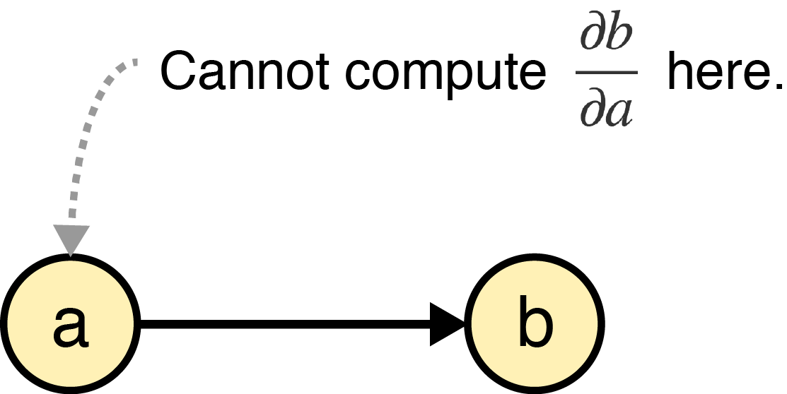
This assertion have to be obvious. If our computational chart represents a function f(a)=bf(a) = bf(a)=b, it is unattainable to compute f′(a)f^{\prime}(a)f′(a) without admission to fff and hence bbb.

In our setup, for all downstream node wjw_jwj​ that depends on a node vvv, it is unattainable to compute ∂wj/∂v\partial w_j / \partial v∂wj​/∂v at node vvv. Therefore, in command to compute ∂f/∂v\partial f / \partial v∂f/∂v, we must decompose the term using the multivariable sequence regulation and continue the another conditions needed to compute ∂f/∂θi\partial f / \partial \theta_i∂f/∂θi​ onward to all node wjw_jwj​ that depends on vvv:

∂f∂θi=(∑j∂f∂wj∂wj∂v⏟Compute on wj)∂v∂θi⏞Pass forward \frac{\partial f}{\partial \theta_i} = \Big( \sum_{j} \frac{\partial f}{\partial w_j} \underbrace{\frac{\partial w_j}{\partial v}}_{\text{Compute on $w_j$}} \Big) \overbrace{\frac{\partial v}{\partial \theta_i}}^{\text{Pass forward}} ∂θi​∂f​=(j∑​∂wj​∂f​Compute on wj​∂v∂wj​​​​)∂θi​∂v​​Pass forward​

We can see that specified an algorithm blows up computationally since we’re onward propagating the same message many times over. For example, if we desire to compute ∂f/∂θi\partial f / \partial \theta_i∂f/∂θi​ and ∂f/∂θk\partial f / \partial \theta_k∂f/∂θk​ anywhere θi\theta_iθi​ and θk\theta_kθk​ are distinct weights in the identical layer, we need to compute ∂v/∂θi\partial v / \partial \theta_i∂v/∂θi​ and ∂v/∂θk\partial v / \partial \theta_k∂v/∂θk​ separately, but all the another conditions are repeated:

∂f∂θi=(∑j(∑k∂f∂zk∂zk∂wj)∂wj∂v)⏞Repeated terms∂v∂θi∂f∂θk=(∑j(∑k∂f∂zk∂zk∂wj)∂wj∂v)∂v∂θk \begin{aligned} \frac{\partial f}{\partial \theta_i} = \overbrace{ \Big( \sum_{j} \Big( \sum_{k} \frac{\partial f}{\partial z_k} \frac{\partial z_k}{\partial w_j} \Big) \frac{\partial w_j}{\partial v} \Big)}^{\text{Repeated terms}} \color{#11accd}{ \frac{\partial v}{\partial \theta_i} } \\ \frac{\partial f}{\partial \theta_k} = \Big( \sum_{j} \Big( \sum_{k} \frac{\partial f}{\partial z_k} \frac{\partial z_k}{\partial w_j} \Big) \frac{\partial w_j}{\partial v} \Big) \color{#bc2612}{ \frac{\partial v}{\partial \theta_k} } \end{aligned} ∂θi​∂f​=(j∑​(k∑​∂zk​∂f​∂wj​∂zk​​)∂v∂wj​​)​Repeated terms​∂θi​∂v​∂θk​∂f​=(j∑​(k∑​∂zk​∂f​∂wj​∂zk​​)∂v∂wj​​)∂θk​∂v​​

Here is a diagram of communication passing the repeated terms:

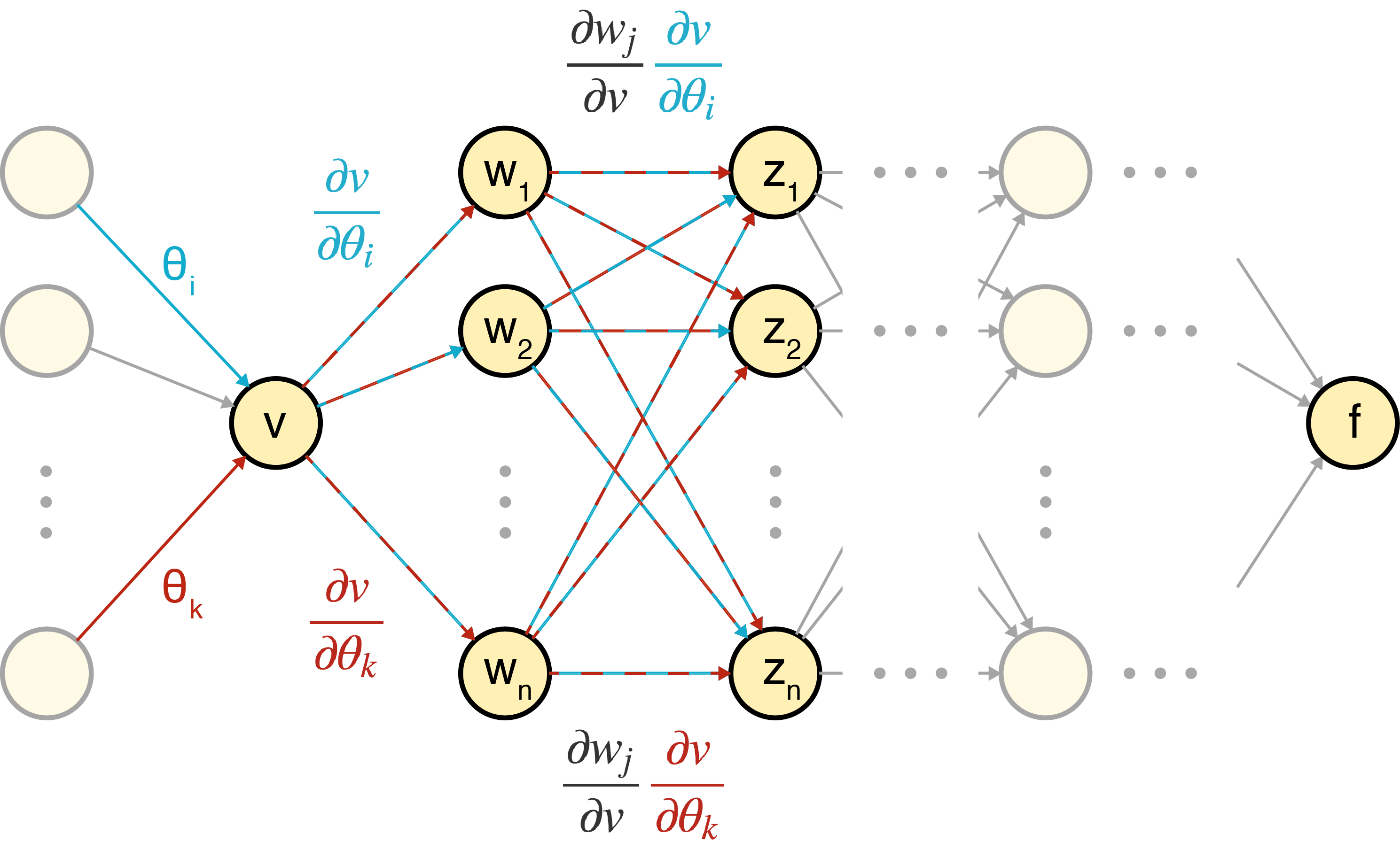
I think the complete diagram is the lynchpin in understanding why backprop goes backwards. This is the key insight: if we already had admission to downstream terms, for example ∂wj/∂v\partial w_j / \partial v∂wj​/∂v, afterward we could communication continue those conditions backwards to node vvv in command to compute ∂f/∂v\partial f / \partial v∂f/∂v. Since all node is fair passing its own local term, the backward continue could be done in linear period alongside regard to the figure of nodes.

A backward pass

I anticipation this clarification it clarifies how you power get to backprop from archetypal principles trying to compute derivatives in a directed acyclic graph. On a stated node bbb that depends on a node aaa, we merely communication continue ∂b/∂a\partial b / \partial a∂b/∂a rear to aaa. The multivariable sequence regulation helps demonstrate the correctness of backprop. For any node vvv alongside downstream weights wjw_jwj​, if vvv merely sums the backwardly propagating messages, it computes its desired derivative:

∂f∂v=∑j∂f∂wj∂wj∂v \frac{\partial f}{\partial v} = \sum_{j} \frac{\partial f}{\partial w_j} \frac{\partial w_j}{\partial v} ∂v∂f​=j∑​∂wj​∂f​∂v∂wj​​

Once you comprehend the chief computational issue backprop solves, I think the norm clarification of backpropagating errors makes much additional sense. This procedure is can be viewed as a resolution to a benevolent of credit project problem: all node tells its upstream neighbors what they did wrong. But the logic the algorithm plant this way is since a naive, onward propagating resolution would have quadratic runtime in the figure of nodes.