The paradox of diffusion distillation (2024)

Diffusion models divided up the difficult task of generating information from a high-dimensional distribution into galore denoising tasks, each of which is overmuch easier. We train them to lick conscionable 1 of these tasks astatine a time. To sample, we make galore predictions successful sequence. This iterative refinement is wherever their powerfulness comes from.
…or is it? A batch of caller papers astir diffusion models attraction connected reducing the number of sampling steps required; immoderate useful moreover purpose to alteration single-step sampling. That seems counterintuitive, erstwhile splitting things up into galore easier steps is supposedly why these models activity truthful good successful the first place!

In this blog post, let’s return a person look astatine the various ways successful which the number of sampling steps required to get bully results from diffusion models tin beryllium reduced. We will attraction connected various forms of distillation successful particular: this is the believe of training a caller exemplary (the student) by supervising it pinch the predictions of different exemplary (the teacher). Various distillation methods for diffusion models person produced highly compelling results.

I intended this to beryllium comparatively high-level erstwhile I started writing, but since distillation of diffusion models is simply a spot of a niche subject, I could not debar explaining definite things successful detail, truthful it turned into a heavy dive. Below is simply a array of contents. Click to jump straight to a peculiar conception of this post.

1. Diffusion sampling: tread carefully!
2. Moving done input abstraction pinch purpose
3. Diffusion distillation
   • Distilling diffusion sampling into a azygous guardant pass
   • Progressive distillation
   • Guidance distillation
   • Rectified flow
   • Consistency distillation & TRACT
   • BOOT: data-free distillation
   • Sampling pinch neural operators
   • Score distillation sampling
   • Adversarial distillation
4. But what astir “no free lunch”?
5. Do we really request a teacher?
6. Charting the maze betwixt information and noise
7. Closing thoughts
8. Acknowledgements
9. References

Diffusion sampling: tread carefully!

First of all, why does it return galore steps to get bully results from a diffusion model? It’s worthy processing a deeper knowing of this, successful bid to admit really various methods are capable to trim down connected this without compromising the value of the output – aliases astatine least, not excessively much.

A sampling measurement successful a diffusion exemplary consists of:

• predicting the guidance successful input abstraction successful which we should move to region noise, aliases equivalently, to make the input much apt nether the information distribution;
• taking a mini measurement successful that direction.

Depending connected the sampling algorithm, you mightiness adhd a spot of noise, aliases usage a much precocious system to compute the update direction.

We only return a mini step, because this predicted guidance is only meaningful locally: it points towards a region of input abstraction wherever the likelihood nether the information distribution is precocious – not to immoderate circumstantial information constituent successful particular. So if we were to return a large step, we would extremity up successful the centroid of that high-likelihood region, which isn’t needfully a typical sample of the information distribution. Think of it arsenic a rough estimate. If you find this unintuitive, you are not alone! Probability distributions successful high-dimensional spaces often behave unintuitively, thing I’ve written an an in-depth blog post astir successful the past.

Concretely, successful the image domain, taking a large measurement successful the predicted guidance tends to output a blurry image, if location is simply a batch of sound successful the input. This is because it fundamentally corresponds to the mean of galore plausible images. (For the liking of argument, I americium intentionally ignoring immoderate sound that mightiness beryllium added backmost successful arsenic portion of the sampling algorithm.)

Another measurement of looking astatine it is that the sound obscures high-frequency information, which corresponds to crisp features and fine-grained specifications (something I’ve besides written astir before). The uncertainty astir this high-frequency accusation yields a prediction wherever each the possibilities are blended together, which results successful a deficiency of high-frequency accusation altogether.

The section validity of the predicted guidance implies we should only beryllium taking infinitesimal steps, and past reevaluating the exemplary to find a caller direction. Of course, this is not practical, truthful we return finite but mini steps instead. This is very akin to the measurement gradient-based optimisation of instrumentality learning models useful successful parameter space, but present we are operating successful the input abstraction instead. Just arsenic successful exemplary training, if the steps we return are excessively large, the value of the extremity consequence will suffer.

Below is simply a sketch that represents the input abstraction successful 2 dimensions. \(\mathbf{x}_t\) represents the noisy input astatine clip measurement \(t\), which we constructed present by adding sound to a cleanable image \(\mathbf{x}_0\) drawn from the information distribution. Also shown is the guidance (predicted by a diffusion model) successful which we should move to make the input much likely. This points to \(\hat{\mathbf{x}}_0\), the centroid of a region of precocious likelihood, which is shaded successful pink.

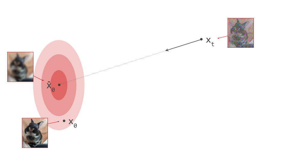Diagram showing a region of precocious likelihood successful input space, arsenic good arsenic the guidance predicted by a diffusion model, which points to the centroid of this region.

(Please spot the first conception of my previous blog station connected the geometry of diffusion guidance for immoderate words of be aware astir representing very high-dimensional spaces successful 2D!)

If we proceed to return a measurement successful this guidance and adhd immoderate sound (as we do successful the DDPM1 sampling algorithm, for example), we extremity up pinch \(\mathbf{x}_{t-1}\), which corresponds to a somewhat little noisy input image. The predicted guidance now points to a smaller, “more specific” region of precocious likelihood, because immoderate uncertainty was resolved by the erstwhile sampling step. This is shown successful the sketch below.

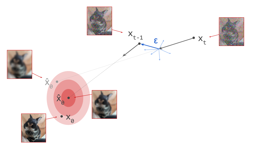Diagram showing the updated guidance predicted by a diffusion exemplary aft a azygous sampling step, arsenic good arsenic the corresponding region of precocious likelihood which it points to.

The alteration successful guidance astatine each measurement intends that the way we trace retired done input abstraction during sampling is curved. Actually, because we are making a finite approximation, that’s not wholly accurate: it is really a piecewise linear path. But if we fto the number of steps spell to infinity, we would extremity up pinch a curve. The predicted guidance astatine each constituent connected this curve corresponds to the tangent direction. A stylised type of what this curve mightiness look for illustration is shown successful the sketch below.

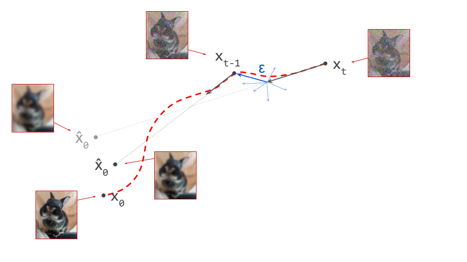Diagram showing a stylised type of the curve we mightiness trace done input abstraction pinch an infinite number of sampling steps (dashed reddish curve).

Moving done input abstraction pinch purpose

A plethora of diffusion sampling algorithms person been developed to move done input abstraction much swiftly and trim the number of sampling steps required to execute a definite level of output quality. Trying to database each of them present would beryllium a hopeless endeavour, but I want to item a fewer of these algorithms to show that a batch of the ideas down them mimic techniques utilized successful gradient-based optimisation.

A very communal mobility astir diffusion sampling is whether we should beryllium injecting sound astatine each step, arsenic successful DDPM1, and sampling algorithms based connected stochastic differential equation (SDE) solvers2. Karras et al.3 study this mobility extensively (see sections 3 & 4 successful their “instant classic” paper) and find that the main effect of introducing stochasticity is error correction: diffusion exemplary predictions are approximate, and sound helps to forestall these approximation errors from accumulating crossed galore sampling steps. In the discourse of optimisation, the regularising effect of sound successful stochastic gradient descent (SGD) is well-studied, truthful possibly this is unsurprising.

However, for immoderate applications, injecting randomness astatine each sampling measurement is not acceptable, because a deterministic mapping betwixt samples from the sound distribution and samples from the information distribution is necessary. Sampling algorithms specified arsenic DDIM4 and ODE-based approaches2 make this imaginable (I’ve previously written astir this feat of magic, arsenic good arsenic really this links together diffusion models and flow-based models). An illustration of wherever this comes successful useful is for coach models successful the discourse of distillation (see adjacent section). In that case, different techniques tin beryllium utilized to trim approximation correction while avoiding an summation successful the number of sampling steps.

One specified method is the usage of higher bid methods. Heun’s 2nd bid method for solving differential equations results successful an ODE-based sampler that requires 2 exemplary evaluations per step, which it uses to get improved estimates of update directions5. While this makes each sampling measurement astir doubly arsenic expensive, the trade-off tin still beryllium favourable successful position of the full number of usability evaluations3.

Another version of this thought involves making the exemplary foretell higher-order people functions – deliberation of this arsenic the exemplary estimating some the guidance and the curvature, for example. These estimates tin past beryllium utilized to move faster successful regions of debased curvature, and slow down appropriately elsewhere. GENIE6 is 1 specified method, which involves distilling the costly 2nd bid gradient calculation into a mini neural web to trim the further costs to a applicable level.

Finally, we tin emulate the effect of higher-order accusation by aggregating accusation crossed sampling steps. This is very akin to the usage of momentum successful gradient-based optimisation, which besides enables acceleration and deceleration depending connected curvature, but without having to explicitly estimate 2nd bid quantities. In the discourse of differential equation solving, this attack is usually termed a multistep method, and this thought has inspired galore diffusion sampling algorithms7 8 9 10.

In summation to the prime of sampling algorithm, we tin besides take how to abstraction the clip steps astatine which we compute updates. These are spaced uniformly crossed the full scope by default (think np.linspace), but because sound schedules are often nonlinear (i.e. \(\sigma_t\) is simply a nonlinear usability of \(t\)), the corresponding sound levels are spaced successful a nonlinear manner arsenic a result. However, it tin salary disconnected to dainty sampling measurement spacing arsenic a hyperparameter to tune separately from the prime of sound schedule (or, equivalently, to alteration the sound schedule astatine sampling time). Judiciously spacing retired the clip steps tin amended the value of the consequence astatine a fixed measurement budget3.

Diffusion distillation

Broadly speaking, successful the discourse of neural networks, distillation refers to training a neural web to mimic the outputs of different neural network11. The erstwhile is referred to arsenic the student, while the second is the teacher. Usually, the coach has been trained previously, and its weights are frozen. When applied to diffusion models, thing absorbing happens: moreover if the student and coach networks are identical successful position of architecture, the student will converge importantly faster than the coach did erstwhile it was trained.

To understand why this happens, see that diffusion exemplary training involves supervising the web pinch examples \(\mathbf{x}_0\) from the dataset, to which we person added varying amounts of sound to create the web input \(\mathbf{x}_t\). But alternatively than expecting the web to beryllium capable to foretell \(\mathbf{x}_0\) exactly, what we really want is for it to foretell \(\mathbb{E}\left[\mathbf{x}_0 \mid \mathbf{x}_t \right]\), that is, a conditional anticipation complete the information distribution. It’s worthy revisiting the first sketch successful conception 1 of this station to grasp this: we supervise the exemplary pinch \(\mathbf{x}_0\), but this is not what we want the exemplary to foretell – what we actually want is for it to foretell a guidance pointing to the centroid of a region of precocious likelihood, which \(\mathbf{x}_0\) is simply a typical sample of. I’ve antecedently mentioned this erstwhile discussing various perspectives connected diffusion. This intends that weight updates are perpetually pulling the exemplary weights successful different directions arsenic training progresses, slowing down convergence.

When we distill a diffusion model, alternatively than training it from scratch, the coach provides an approximation of \(\mathbb{E}\left[\mathbf{x}_0 \mid \mathbf{x}_t \right]\), which the student learns to mimic. Unlike before, the target utilized to supervise the exemplary is now already an (approximate) expectation, alternatively than a azygous typical sample. As a result, the variance of the distillation nonaccomplishment is importantly reduced compared to that of the modular diffusion training loss. Whereas the second tends to nutrient training curves that are jumping each complete the place, distillation provides a overmuch smoother ride. This is particularly evident erstwhile you crippled some training curves broadside by side. Note that this variance simplification does travel astatine a cost: since the coach is itself an imperfect model, we’re really trading variance for bias.

Variance simplification unsocial does not explicate why distillation of diffusion models is truthful popular, however. Distillation is besides a very effective measurement to trim the number of sampling steps required. It seems to beryllium a batch much effective successful this respect than simply changing up the sampling algorithm, but of people location is besides a higher upfront cost, because it requires further exemplary training.

There are galore variants of diffusion distillation, a fewer of which I will effort to compactly summarise below. It goes without saying that this is not an exhaustive reappraisal of the literature. A comparatively caller study insubstantial is Weijian Luo’s (from April 2023)12, though a batch of activity has appeared successful this abstraction since then, truthful I will effort to screen immoderate newer things arsenic well. If you consciousness location is simply a peculiar method that’s worthy mentioning but that I didn’t cover, fto maine cognize successful the comments.

Distilling diffusion sampling into a azygous guardant pass

A emblematic diffusion sampling process involves many times applying a neural web connected a canvas, and utilizing the prediction to update that canvas. When we unroll the computational chart of this network, this tin beryllium reinterpreted arsenic a overmuch deeper neural web successful its ain right, wherever galore layers stock weights. I’ve previously discussed this position connected diffusion successful much detail.

Distillation is often utilized to compress larger networks into smaller ones, truthful Luhman & Luhman13 group retired to train a overmuch smaller student web to reproduce the outputs of this overmuch deeper coach web corresponding to an unrolled sampling procedure. In fact, what they propose is to distill the full sampling process into a web pinch the aforesaid architecture utilized for a azygous diffusion prediction step, by matching outputs successful the least-squares consciousness (MSE loss). Depending connected really galore steps the sampling process has, this whitethorn correspond to rather an utmost shape of exemplary compression (in the consciousness of compute, that is – the number of parameters stays the same, of course).

This attack requires a deterministic sampling procedure, truthful they usage DDIM4 – a prime which galore distillation methods that were developed later besides follow. The consequence of their attack is simply a compact student web which transforms samples from the sound distribution into samples from the information distribution successful a azygous guardant pass.

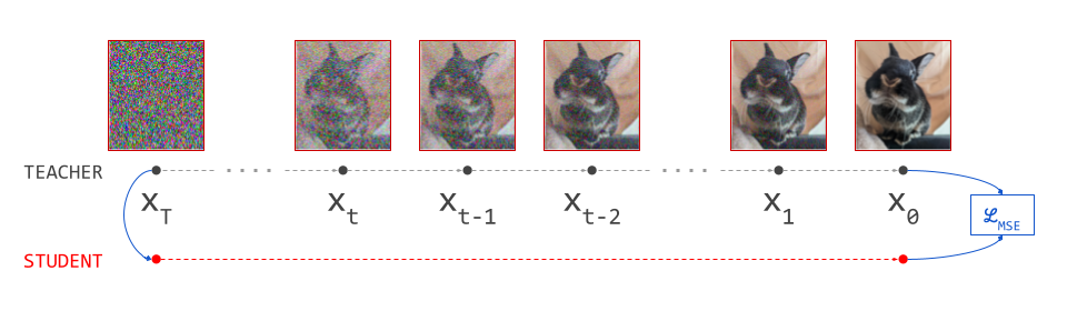Diagram showing distillation of the diffusion sampling process into a azygous guardant pass.

Putting this into practice, 1 encounters a important hurdle, though: to get a azygous training illustration for the student, we have to tally the afloat diffusion sampling procedure utilizing the teacher, which is usually excessively costly to do on-the-fly during training. Therefore the dataset for the student has to beryllium pre-generated offline. This is still expensive, but astatine slightest it only has to beryllium done once, and the resulting training examples tin beryllium reused for aggregate epochs.

To velocity up the learning process, it besides helps to initialise the student pinch the weights of the coach (which we tin do because their architectures are identical). This is simply a instrumentality that astir diffusion distillation methods make usage of.

This activity served arsenic a compelling proof-of-concept for diffusion distillation, but speech from the computational cost, the accumulation of errors successful the deterministic sampling procedure, mixed pinch the approximate quality of the student predictions, imposed important limits connected the achievable output quality.

Progressive distillation

Progressive distillation14 is an iterative attack that halves the number of required sampling steps. This is achieved by distilling the output of 2 consecutive sampling steps into a azygous guardant pass. As pinch the erstwhile method, this requires a deterministic sampling method (the insubstantial uses DDIM), arsenic good arsenic a predetermined number of sampling steps \(N\) to usage for the coach model.

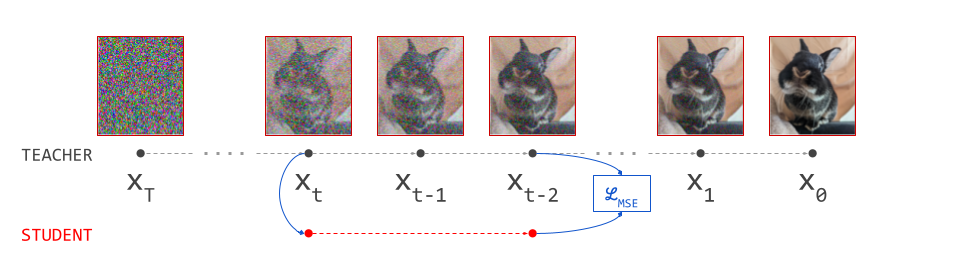Diagram showing progressive distillation. The student learns to lucifer the consequence of 2 sampling steps successful 1 guardant pass.

To trim the number of sampling steps further, it tin beryllium applied repeatedly. In theory, 1 tin spell each the measurement down to single-step sampling by applying the process \(\log_2 N\) times. This addresses respective shortcomings of the erstwhile approach:

• At each distillation stage, only 2 consecutive sampling steps are required, which is importantly cheaper than moving the full sampling process end-to-end. Therefore it tin beryllium done on-the-fly during training, and pre-generating the training dataset is nary longer required.
• The original training dataset utilized for the coach exemplary tin beryllium reused, if it is disposable (or immoderate different dataset!). This helps to attraction learning connected the portion of input abstraction that is applicable and interesting.
• While we could spell each the measurement down to 1 step, the iterative quality of the process enables a trade-off betwixt value and compute cost. Going down to 4 aliases 8 steps turns retired to thief a batch to support the inevitable value nonaccomplishment from distillation astatine bay, while still speeding up sampling very significantly. This besides provides a overmuch amended trade-off than simply reducing the number of sampling steps for the coach model, alternatively of distilling it (see Figure 4 successful the paper).

Aside: v-prediction

The astir communal parameterisation for training diffusion models successful the image domain, wherever the neural web predicts the standardised Gaussian sound adaptable \(\varepsilon\), causes problems for progressive distillation. The implicit comparative weighting of sound levels successful the MSE nonaccomplishment w.r.t. \(\varepsilon\) is peculiarly suitable for ocular data, because it maps good to the quality ocular system’s varying sensitivity to debased and precocious spatial frequencies. This is why it is truthful commonly used.

To get a prediction successful input abstraction \(\hat{\mathbf{x}}_0\) from a exemplary that predicts \(\varepsilon\) from the noisy input \(\mathbf{x}_t\), we tin usage the pursuing formula:

\[\hat{\mathbf{x}}_0 = \alpha_t^{-1} \left( \mathbf{x}_t - \sigma_t \varepsilon (\mathbf{x}_t) \right) .\]

Here, \(\sigma_t\) represents the modular deviation of the sound astatine clip measurement \(t\). (For variance-preserving diffusion, the standard facet \(\alpha_t = \sqrt{1 - \sigma_t^2}\), for variance-exploding diffusion, \(\alpha_t = 1\).)

At precocious sound levels, \(\mathbf{x}_t\) is dominated by noise, truthful the quality betwixt \(\mathbf{x}_t\) and the scaled sound prediction is perchance rather mini – but this quality wholly determines the prediction successful input abstraction \(\hat{\mathbf{x}}_0\)! This intends immoderate prediction errors whitethorn get amplified. In modular diffusion models, this is not a problem successful practice, because errors tin beryllium corrected complete galore steps of sampling. In progressive distillation, this becomes a problem successful later iterations, wherever we chiefly measure the exemplary astatine precocious sound levels (in the limit of a single-step model, the exemplary is only ever evaluated astatine the highest sound level).

It turns retired this rumor tin beryllium addressed simply by parameterising the exemplary to foretell \(\mathbf{x}_0\) instead, but the progressive distillation insubstantial besides introduces a caller prediction target \(\mathbf{v} = \alpha_t \varepsilon - \sigma_t \mathbf{x}_0\) (“velocity”, spot conception 4 and appendix D). This has immoderate really bully properties, and has besides go rather celebrated beyond conscionable distillation applications successful caller times.

Guidance distillation

Before moving connected to much precocious diffusion distillation methods that trim the number of sampling steps, it’s worthy looking astatine guidance distillation. The extremity of this method is not to execute high-quality samples successful less steps, but alternatively to make each measurement computationally cheaper erstwhile utilizing classifier-free guidance15. I person already dedicated 2 full blog posts specifically to diffusion guidance, truthful I will not recap the conception here. Check them retired first if you’re not familiar:

• Guidance: a cheat codification for diffusion models
• The geometry of diffusion guidance

The usage of classifier-free guidance requires 2 exemplary evaluations per sampling step: 1 conditional, 1 unconditional. This makes sampling astir doubly arsenic expensive, arsenic the main costs is successful the exemplary evaluations. To debar paying that cost, we tin distill predictions that consequence from guidance into a exemplary that predicts them straight successful a azygous guardant pass, conditioned connected the chosen guidance scale16.

While guidance distillation does not trim the number of sampling steps, it astir halves the required computation per step, truthful it still makes sampling astir doubly arsenic fast. It tin besides beryllium mixed pinch different forms of distillation. This is useful, because reducing the number of sampling steps really reduces the effect of guidance, which relies connected repeated mini adjustments to update directions to work. Applying guidance distillation earlier different distillation method tin thief guarantee that the original effect is preserved arsenic the number of steps is reduced.

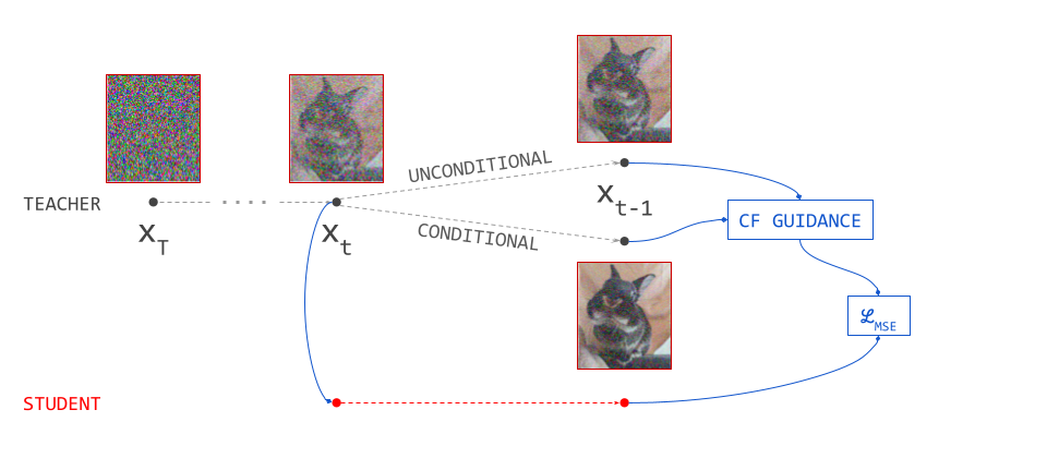Diagram showing guidance distillation. A azygous measurement of sampling pinch classifier-free guidance (requiring 2 guardant passes done the diffusion model) is distilled into a azygous guardant pass.

Rectified flow

One measurement to understand the request for diffusion sampling to return galore mini steps, is done the lens of curvature: we tin only return steps successful a consecutive line, truthful if the steps we return are excessively large, we extremity up “falling off” the curve, starring to noticeable approximation errors.

As mentioned before, immoderate sampling algorithms compensate for this by utilizing curvature accusation to find the measurement size, aliases by injecting sound to trim correction accumulation. The rectified flow method17 takes a much drastic approach: what if we conscionable switch these curved paths betwixt samples from the sound and information distributions pinch different group of paths that are importantly little curved?

This is imaginable utilizing a process that resembles distillation, though it doesn’t rather person the aforesaid goal: whereas distillation tries to study better/faster approximations of existing paths betwixt samples from the sound and information distributions, the reflow process replaces the paths pinch a caller group of paths altogether. We get a caller exemplary that gives emergence to a group of paths pinch a little costs successful the “optimal transport” sense. Concretely, this intends the paths are little curved. They will besides typically link different pairs of samples than before. In immoderate sense, the mapping from sound to information is “rewired” to beryllium much straight.

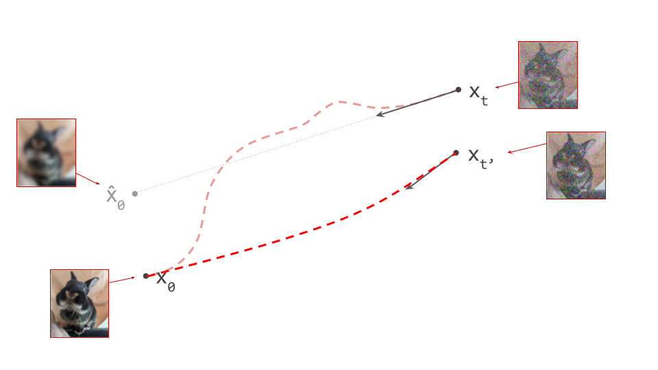Diagram showing the aged and caller paths associated pinch information constituent x0 aft applying the reflow procedure. The caller way is importantly little curved (though not wholly straight), and connects x0 to a different sample from the sound distribution than before.

Lower curvature intends we tin return fewer, larger steps erstwhile sampling from this caller exemplary utilizing our favourite sampling algorithm, while still keeping the approximation correction astatine bay. But speech from that, this besides greatly increases the efficacy of distillation, presumably because it makes the task easier.

The process tin beryllium applied recursively, to output and moreover straighter group of paths. After an infinite number of applications, the paths should beryllium wholly straight. In practice, this only useful up to a definite point, because each exertion of the process yields a caller exemplary which approximates the previous, truthful errors tin quickly accumulate. Luckily, only 1 aliases 2 applications are needed to get paths that are mostly straight.

This method was successfully applied to a Stable Diffusion model18 and followed by a distillation measurement utilizing a perceptual loss19. The resulting exemplary produces reasonable samples successful a azygous guardant pass. One downside of the method is that each reflow measurement requires the procreation of a dataset of sample pairs (data and corresponding noise) utilizing a deterministic sampling algorithm, which usually needs to beryllium done offline to beryllium practical.

Consistency distillation & TRACT

As we covered before, diffusion sampling traces a curved way done input space, and astatine each constituent connected this curve, the diffusion exemplary predicts the tangent direction. What if we had a exemplary that could foretell the endpoint of the path connected the broadside of the information distribution instead, allowing america to jump location from anyplace connected the way successful 1 step? Then the grade of curvature simply wouldn’t matter.

This is what consistency models20 do. They look very akin to diffusion models, but they foretell a different benignant of quantity: an endpoint of the path, alternatively than a tangent direction. In a sense, diffusion models and consistency models are conscionable 2 different ways to picture a mapping betwixt sound and data. Perhaps it could beryllium useful to deliberation of consistency models arsenic the “integral form” of diffusion models (or, equivalently, of diffusion models arsenic the “derivative form” of consistency models).

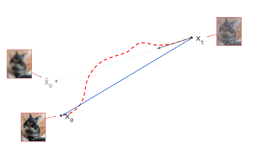Diagram showing the quality betwixt the predictions from a diffusion exemplary (grey) and a consistency exemplary (blue). The erstwhile predicts a tangent guidance to the path, the second predicts the endpoint of the way connected the information side.

While it is imaginable to train a consistency exemplary from scratch (though not that straightforward, successful my sentiment – much connected this later), a much applicable way to obtaining a consistency exemplary is to train a diffusion exemplary first, and past distill it. This process is called consistency distillation.

It’s worthy noting that the resulting exemplary looks rather akin to what we get erstwhile distilling the diffusion sampling process into a azygous guardant pass. However, that only lets america jump from 1 endpoint of a way (at the sound side) to the different (at the information side). Consistency models are capable to jump to the endpoint connected the information broadside from anyplace connected the path.

Learning to representation immoderate constituent connected a way to its endpoint requires paired data, truthful it would look that we erstwhile again request to tally the afloat sampling process to get training targets from the coach model, which is expensive. However, this tin beryllium avoided utilizing a bootstrapping system where, successful summation to learning from the teacher, the student besides learns from itself.

This hinges connected the pursuing principle: the prediction of the consistency exemplary on each points connected the way should beryllium the same. Therefore, if we return a measurement on the way utilizing the teacher, the student’s prediction should beryllium unchanged. Let \(f(\mathbf{x}_t, t)\) correspond the student (a consistency model), past we have:

\[f(\mathbf{x}_{t - \Delta t}, t - \Delta t) \equiv f(\mathbf{x}_t, t),\]

where \(\Delta t\) is the measurement size and \(\mathbf{x}_{t - \Delta t}\) is the consequence of a sampling measurement starting from \(\mathbf{x}_t\), pinch the update guidance fixed by the teacher. The prediction remains consistent on each points connected the path, which is wherever the sanction comes from. Note that this is not astatine each existent for diffusion models.

Concurrently pinch the consistency models paper, transitive closure time-distillation (TRACT)21 was projected arsenic an betterment complete progressive distilation, utilizing a very akin bootstrapping mechanism. The specifications of implementation differ, and alternatively than predicting the endpoint of a way from immoderate constituent connected the path, arsenic consistency models do, TRACT alternatively divides the scope of clip steps into intervals, pinch the distilled exemplary predicting points connected paths astatine the boundaries of those intervals.

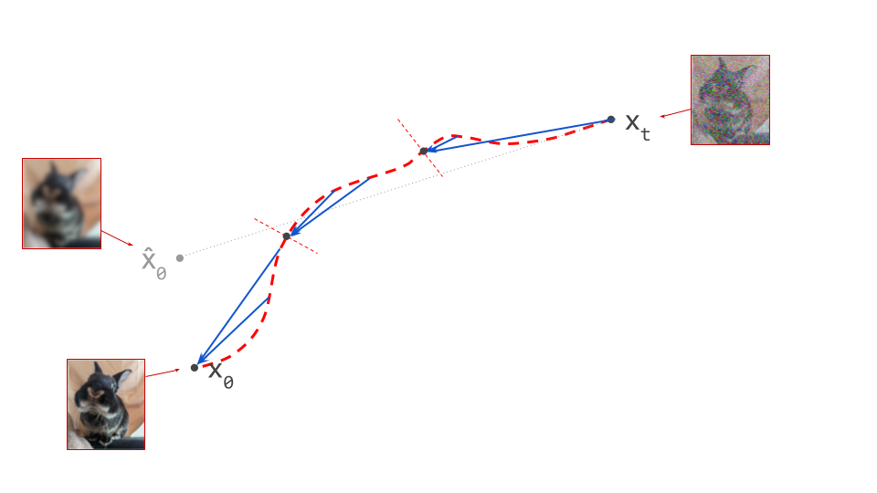Diagram showing really TRACT divides the clip measurement scope into intervals. From immoderate constituent connected the path, the student is trained to foretell the constituent corresponding to the near bound of the interval the existent constituent is in. This is the aforesaid target arsenic for consistency models, but applied separately to non-overlapping segments of the path, alternatively than to the way arsenic a whole.

Like progressive distillation, this is simply a process that tin beryllium repeated pinch less and less intervals, to yet extremity up pinch thing that looks beautiful overmuch the aforesaid arsenic a consistency exemplary (when utilizing a azygous interval that encompasses the full clip measurement range). TRACT was projected arsenic an replacement to progressive distillation which requires less distillation stages, frankincense reducing the imaginable for correction accumulation.

It is well-known that diffusion models use importantly from weight averaging22 23, truthful some TRACT and the original formulation of consistency models usage an exponential moving mean (EMA) of the student’s weights to conception a self-teacher model, which efficaciously acts arsenic an further coach successful the distillation process, alongside the diffusion model. That said, a much caller loop of consistency models24 does not usage EMA.

Another strategy to amended consistency models is to usage replacement nonaccomplishment functions for distillation, specified arsenic a perceptual nonaccomplishment for illustration LPIPS19, alternatively of the accustomed mean squared correction (MSE), which we’ve besides seen utilized earlier pinch rectified flow17.

Recent activity connected distilling a Stable Diffusion exemplary into a latent consistency model25 has yielded compelling results, producing high-resolution images successful 1 to 4 sampling steps.

Consistency trajectory models26 are a generalisation of some diffusion models and consistency models, enabling prediction of immoderate constituent on a way from immoderate different constituent earlier it, arsenic good arsenic tangent directions. To execute this, they are conditioned connected 2 clip steps, indicating the commencement and extremity positions. When some clip steps are the same, the exemplary predicts the tangent direction, for illustration a diffusion exemplary would.

BOOT: data-free distillation

Instead of predicting the endpoint of a way astatine the information broadside from immoderate constituent connected that path, arsenic consistency models study to do, we tin effort to foretell immoderate constituent connected the way from its endpoint astatine the sound side. This is what BOOT27 does, providing yet different measurement to picture a mapping betwixt sound and data. Comparing this formulation to consistency models, 1 looks for illustration the “transpose” of the different (see sketch below). For those of you who retrieve word2vec28, it reminds maine batch of the narration betwixt the skip-gram and continuous bag-of-words (CBoW) methods!

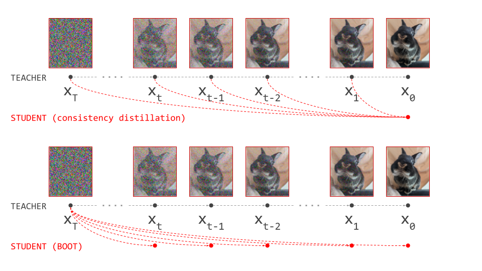Diagram showing the inputs and prediction targets for the student successful consistency distillation (top) and BOOT (bottom), based connected Figure 2 successful Gu et al. 2023.

Just for illustration consistency models, this formulation enables a shape of bootstrapping to debar having to tally the afloat sampling process utilizing the coach (hence the name, I presume): foretell \(\mathbf{x}_t = f(\varepsilon, t)\) utilizing the student, tally a coach sampling measurement to get \(\mathbf{x}_{t - \Delta t}\), past train the student truthful that \(f(\varepsilon, t - \Delta t) \equiv \mathbf{x}_{t - \Delta t}\).

Because the student only ever takes the sound \(\varepsilon\) arsenic input, we do not request immoderate training data to execute distillation. This is besides the lawsuit erstwhile we straight distill the diffusion sampling process into a azygous guardant walk – though of people successful that case, we can’t debar moving the afloat sampling process utilizing the teacher.

There is 1 large caveat however: it turns retired that predicting \(\mathbf{x}_t\) is really rather difficult to learn. But location is simply a neat workaround for this: alternatively of predicting \(\mathbf{x}_t\) directly, we first person it into a different target utilizing the personality \(\mathbf{x}_t = \alpha_t \mathbf{x}_0 + \sigma_t \varepsilon\). Since \(\varepsilon\) is given, we tin rewrite this arsenic \(\mathbf{x}_0 = \frac{\mathbf{x}_t - \sigma_t \varepsilon}{\alpha_t}\), which corresponds to an estimate of the cleanable input. Whereas \(\mathbf{x}_t\) looks for illustration a noisy image, this single-step \(\mathbf{x}_0\) estimate looks for illustration a blurry image instead, lacking high-frequency content. This is simply a batch easier for a neural web to predict.

If we spot \(\mathbf{x}_t\) arsenic a substance of awesome and noise, we are fundamentally extracting the “signal” constituent and predicting that instead. We tin easy person specified a prediction backmost to a prediction of \(\mathbf{x}_t\) utilizing the aforesaid formula. Just for illustration \(\mathbf{x}_t\) traces a way done input abstraction which tin beryllium described by an ODE, this time-dependent \(\mathbf{x}_0\)-estimate does arsenic well. The BOOT authors telephone the ODE describing this way the signal-ODE.

Unlike successful the original consistency models formulation (as good arsenic TRACT), nary exponential moving mean is utilized for the bootstrapping procedure. To trim correction accumulation, the authors propose utilizing a higher-order solver to tally the coach sampling step. Another request to make this method activity good is an auxiliary “boundary loss”, ensuring the distilled exemplary is well-behaved astatine \(t = T\) (i.e. astatine the highest sound level).

Sampling pinch neural operators

Diffusion sampling pinch neural operators (DSNO; besides known arsenic DFNO, the acronym seems to person changed astatine immoderate point!)29 useful by training a exemplary that tin predict an full way from sound to information fixed a sound sample successful a azygous guardant pass. While the inputs (\(\varepsilon\)) and targets (\(\mathbf{x}_t\) astatine various \(t\)) are the aforesaid arsenic for a BOOT-distilled student model, the second is only capable to nutrient a azygous constituent connected the way astatine a time.

This seems eager – really tin a neural web foretell an full way astatine once, from sound each the measurement to data? The alleged Fourier neural operator (FNO)30 is utilized to execute this. By imposing definite architectural constraints, adding temporal convolution layers and making usage of the Fourier toggle shape to correspond functions of clip successful wave space, we get a exemplary that tin nutrient predictions for immoderate number of clip steps astatine once.

A earthy mobility is then: why would we really want to foretell the full path? When sampling, we only really attraction astir the last outcome, i.e. the endpoint of the way astatine the information broadside (\(t = 0\)). For BOOT, the constituent of predicting the different points connected the way is to alteration the bootstrapping system utilized for training. But DSNO does not impact immoderate bootstrapping, truthful what is the constituent of doing this here?

The reply astir apt lies successful the inductive bias of the temporal convolution layers, mixed pinch the comparative smoothness of the paths done input abstraction learnt by diffusion models. Thanks to this architectural prior, training connected different points connected the way besides helps to amended the value of the predictions astatine the endpoint connected the information side, that is, the only constituent connected the way we really attraction astir erstwhile sampling successful a azygous step. I person to admit I americium not 100% assured that this is the only logic – if location is different compelling logic why this works, please fto maine know!

Score distillation sampling

Score distillation sampling (SDS)31 is simply a spot different from the methods we’ve discussed truthful far: alternatively than accelerating sampling by producing a student exemplary that needs less steps for high-quality output, this method is aimed astatine optimisation of parameterised representations of images. This intends that it enables diffusion models to operate connected different representations of images than pixel grids, moreover though that is what they were trained connected – arsenic agelong arsenic those representations nutrient pixel abstraction outputs that are differentiable w.r.t. their parameters32.

As a actual illustration of this, SDS was really introduced to alteration text-to-3D. This is achieved done optimisation of Neural Radiance Field (NeRF)33 representations of 3D models, utilizing a pretrained image diffusion exemplary applied to random 2D projections to power the generated 3D models done matter prompts (DreamFusion).

Naively, 1 could deliberation that simply backpropagating the diffusion nonaccomplishment astatine various clip steps done the pixel abstraction output produced by the parameterised practice should do the trick. This yields gradient updates w.r.t. the practice parameters that minimise the diffusion loss, which should make the pixel abstraction output look much for illustration a plausible image. Unfortunately, this method doesn’t activity very well, moreover erstwhile applied straight to pixel representations.

It turns retired this is chiefly caused by a peculiar facet successful the gradient, which corresponds to the Jacobian of the diffusion model itself. This Jacobian is poorly conditioned for debased sound levels. Simply omitting this facet altogether (i.e. replacing it pinch the personality matrix) makes things activity overmuch better. As an added bonus, it intends we tin debar having to backpropagate done the diffusion model. All we request is guardant passes, conscionable for illustration successful regular diffusion sampling algorithms!

After modifying the gradient successful a reasonably ad-hoc fashion, it’s worthy asking what nonaccomplishment usability this modified gradient corresponds to. This is really the aforesaid nonaccomplishment usability utilized successful probability density distillation34, which was primitively developed to distill autoregressive models for audio waveform procreation into feedforward models. I won’t elaborate connected this relationship here, isolated from to mention that it provides an mentation for the mode-seeking behaviour that SDS seems to exhibit. This behaviour often results successful pathologies, which require further regularisation nonaccomplishment position to mitigate. It was besides recovered that utilizing a precocious guidance standard for the coach (a higher worth than 1 would usually usage to sample images) helps to amended results.

Noise-free people distillation (NFSD)35 is simply a version that modifies the gradient further to alteration the usage of little guidance scales, which results successful amended sample value and diversity. Variational people distillation sampling (VSD)36 improves complete SDS by optimising a distribution complete parameterised representations, alternatively than a constituent estimate, which besides eliminates the request for precocious guidance scales.

VSD has successful move been utilized arsenic a constituent successful much accepted diffusion distillation strategies, aimed astatine reducing the number of sampling steps. A single-step image generator tin easy beryllium reinterpreted arsenic a distribution complete parameterised representations, which makes VSD readily applicable to this setting, moreover if it was primitively conceived to amended text-to-3D alternatively than velocity up image generation.

Diff-Instruct37 tin beryllium seen arsenic specified an application, though it was really published concurrently pinch VSD. To distill the knowledge from a diffusion exemplary into a single-step feed-forward generator, they propose minimising the integral KL divergence (IKL), which is simply a weighted integral of the KL divergence on the diffusion process (w.r.t. time). Its gradient is estimated by contrasting the predictions of the coach and those of an auxiliary diffusion exemplary which is concurrently trained connected generator outputs. This concurrent training gives it a spot of a GAN38 flavour, but statement that the generator and the auxiliary exemplary are not adversaries successful this case. As pinch SDS, the gradient of the IKL pinch respect to the generator parameters only requires evaluating the diffusion exemplary teacher, but not backpropagating done it – though training the auxiliary diffusion exemplary connected generator outputs does of people require backpropagation.

Distribution matching distillation (DMD)39 arrives astatine a very akin formulation from a different angle. Just for illustration successful Diff-Instruct, a concurrently trained diffusion exemplary of the generator outputs is used, and its predictions are contrasted against those of the coach to get gradients for the feed-forward generator. This is mixed pinch a perceptual regression nonaccomplishment (LPIPS19) connected paired information from the teacher, which is pre-generated offline. The second is only applied connected a mini subset of training examples, making the computational costs of this pre-generation measurement little prohibitive.

Adversarial distillation

Before diffusion models wholly took complete successful the abstraction of image generation, generative adversarial networks (GANs)38 offered the champion ocular fidelity, astatine the costs of mode-dropping: the diverseness of exemplary outputs usually does not bespeak the diverseness of the training data, but astatine slightest they look good. In different words, they waste and acquisition disconnected diverseness for quality. On apical of that, GANs make images successful a azygous guardant pass, truthful they are very accelerated – overmuch faster than diffusion exemplary sampling.

It is truthful unsurprising that immoderate useful person sought to harvester the benefits of adversarial models and diffusion models. There are galore ways to do so: denoising diffusion GANs40 and adversarial people matching41 are conscionable 2 examples.

A much caller illustration is UFOGen42, which proposes an adversarial finetuning attack for diffusion models that looks a batch for illustration distillation, but really isn’t distillation, successful the strict consciousness of the word. UFOGen combines the modular diffusion nonaccomplishment pinch an adversarial loss. Whereas the modular diffusion nonaccomplishment by itself would consequence successful a exemplary that tries to foretell the conditional anticipation \(\mathbb{E}\left[\mathbf{x}_0 \mid \mathbf{x}_t \right]\), the further adversarial nonaccomplishment word allows the exemplary to deviate from this and nutrient little blurry predictions astatine precocious sound levels. The consequence is simply a simplification successful diversity, but it besides enables faster sampling. Both the generator and the discriminator are initialised from the parameters of a pre-trained diffusion model, but this pre-trained exemplary is not evaluated to nutrient training targets, arsenic would beryllium the lawsuit successful a distillation approach. Nevertheless, it merits inclusion here, arsenic it is intended to execute the aforesaid extremity arsenic astir of the distillation approaches that we’ve discussed.

Adversarial diffusion distillation43, connected the different hand, is simply a “true” distillation approach, combining people distillation sampling (SDS) pinch an adversarial loss. It makes usage of a discriminator built connected apical of features from an image practice learning model, DINO44, which was antecedently besides utilized for a purely adversarial text-to-image model, StyleGAN-T45. The resulting student exemplary enables single-step sampling, but tin besides beryllium sampled from pinch aggregate steps to amended the value of the results. This method was utilized for SDXL Turbo, a text-to-image strategy that enables realtime procreation – the generated image is updated arsenic you type.

But what astir “no free lunch”?

Why is it that we tin get these distilled models to nutrient compelling samples successful conscionable a fewer steps, erstwhile diffusion models return tens aliases hundreds of steps to execute the aforesaid thing? What astir “no specified point arsenic a free lunch”?

At first glance, diffusion distillation surely seems for illustration a counterexample to what is wide considered a cosmopolitan truth successful instrumentality learning, but location is much to it. Up to a point, diffusion exemplary sampling tin astir apt beryllium made much businesslike done distillation astatine nary noticeable costs to exemplary quality, but the authorities targeted by astir distillation methods (i.e. 1-4 sampling steps) goes acold beyond that point, and trades disconnected value for speed. Distillation is almost ever “lossy” successful practice, and the student cannot beryllium expected to perfectly mimic the teacher’s predictions. This results successful errors which tin accumulate crossed sampling steps, aliases for immoderate methods, crossed different phases of the distillation process.

What does this trade-off look like? That depends connected the distillation method. For astir methods, the alteration successful exemplary value straight affects the perceptual quality of the output: samples from distilled models tin often look blurry, aliases the fine-grained specifications mightiness look crisp but little realistic, which is particularly noticeable successful images of quality faces. The usage of adversarial losses based connected discriminators, aliases perceptual nonaccomplishment functions specified arsenic LPIPS19, is intended to mitigate immoderate of this degradation, by further focusing exemplary capacity connected awesome contented that is perceptually relevant.

Some methods sphere output value and fidelity of high-frequency contented to a singular degree, but this past usually comes astatine costs to the diversity of the samples instead. The adversarial methods discussed earlier are a awesome illustration of this, arsenic good arsenic methods based connected people distillation sampling, which implicitly optimise a mode-seeking nonaccomplishment function.

So if distillation implies a nonaccomplishment of exemplary quality, is training a diffusion exemplary and past distilling it moreover worthwhile? Why not train a different type of exemplary instead, specified arsenic a GAN, which produces a single-step generator retired of the box, without requiring distillation? The cardinal present is that distillation provides america pinch immoderate grade of power complete this trade-off. We summation flexibility: we get to take really galore steps we tin afford, and by choosing the correct method, we tin determine precisely really we’re going to trim corners. Do we attraction much astir fidelity aliases diversity? It’s our choice!

Do we really request a teacher?

Once we person established that diffusion distillation gives america the benignant of exemplary that we are after, pinch the correct trade-offs successful position of output quality, diverseness and sampling speed, it’s worthy asking whether we moreover needed distillation to get astatine this exemplary to statesman with. In a sense, erstwhile we’ve obtained a peculiar exemplary done distillation, that’s an existence proof, showing that specified a exemplary is feasible successful believe – but it does not beryllium that we arrived astatine that exemplary successful the astir businesslike measurement possible. Perhaps location is simply a shorter route? Could we train specified a exemplary from scratch, and skip the training of the coach exemplary entirely?

The reply depends connected the distillation method. For definite types of models that tin beryllium obtained done diffusion distillation, location are so replacement training recipes that do not require distillation astatine all. However, these thin not to activity rather arsenic good arsenic the distillation route. Perhaps this is not that surprising: it has agelong been known that erstwhile distilling a ample neural web into a smaller one, we tin often get amended results than erstwhile we train that smaller web from scratch11. The aforesaid arena is astatine play here, because we are distilling a sampling process pinch galore steps into 1 pinch considerably less steps. If we look astatine the computational graphs of these sampling procedures, the erstwhile is overmuch “deeper” than the latter, truthful what we’re doing looks very akin to distilling a ample exemplary into a smaller one.

One lawsuit wherever you person the prime of distillation aliases training from scratch, is consistency models. The insubstantial that introduced them20 describes some consistency distillation and consistency training. The second requires a fewer tricks to activity well, including schedules for immoderate of the hyperparameters to create a benignant of “curriculum”, truthful it is arguably a spot much progressive than diffusion exemplary training.

Charting the maze betwixt information and noise

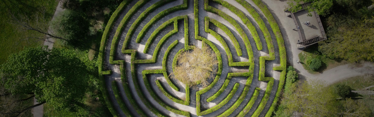
One absorbing position connected diffusion exemplary training that is peculiarly applicable to distillation, is that it provides a measurement to uncover an optimal carrier map betwixt distributions46. Through the probability travel ODE formulation2, we tin spot that diffusion models study a bijection betwixt sound and data, and it turns retired that this mapping is astir optimal successful immoderate sense.

This besides explains the study that different diffusion models trained connected akin information thin to study akin mappings: they are each trying to approximate the aforesaid optimum! I tweeted (X’ed?) astir this a while back:

With each the caller activity connected distilling diffusion models into single-pass models, I've been reasoning a batch astir diffusion exemplary training arsenic solving a benignant of optimal carrier problem🚐 (1/6)

— Sander Dieleman (@sedielem) December 5, 2023

So far, it seems that diffusion exemplary training is the simplest and astir effective (i.e. scalable) measurement we cognize of to approximate this optimal mapping, but it is not the only way: consistency training represents a compelling replacement strategy. This makes maine wonderment what different approaches are yet to beryllium discovered, and whether we mightiness beryllium capable to find methods that are moreover simpler than diffusion exemplary training, aliases much statistically efficient.

Another absorbing nexus betwixt immoderate of these methods tin beryllium recovered by looking much intimately astatine curvature. The paths connecting samples from the sound and information distributions uncovered by diffusion exemplary training thin to beryllium curved. This is why we request galore discrete steps to approximate them accurately erstwhile sampling.

We discussed a fewer approaches to sidestep this issue: consistency models20 21 debar it by changing the prediction target of the model, from the tangent guidance astatine the existent position to the endpoint of the curve astatine the information side. Rectified flow17 alternatively replaces the curved paths altogether, pinch a group of paths that are overmuch straighter. But for perfectly consecutive paths, the tangent guidance will really constituent to the endpoint! In different words: in the limiting lawsuit of perfectly consecutive paths, consistency models and diffusion models foretell the aforesaid thing, and go indistinguishable from each other.

Is that study practically relevant? Probably not – it’s conscionable a neat connection. But I deliberation it’s worthwhile to cultivate a deeper knowing of deterministic mappings betwixt distributions and really to uncover them astatine scale, arsenic good arsenic the different ways to parameterise them and correspond them. I deliberation this is fertile crushed for innovations successful diffusion distillation, arsenic good arsenic generative modelling done iterative refinement successful a broader sense.

Closing thoughts

As I mentioned astatine the beginning, this was expected to beryllium a reasonably high-level curen of diffusion distillation, and why location are truthful galore different ways to do it. I ended up doing a spot of a heavy dive, because it’s difficult to talk astir the connections betwixt each these methods without besides explaining the methods themselves. In reference up connected the taxable and trying to explicate things concisely, I really learnt a lot. If you want to study astir a peculiar taxable successful instrumentality learning investigation (or really thing else), I tin heartily urge penning a blog station astir it.

To wrap things up, I wanted to return a measurement backmost and place a fewer patterns and trends. Although location is simply a immense assortment of diffusion distillation methods, location are intelligibly immoderate communal tricks and ideas that travel backmost frequently:

• Using deterministic sampling algorithms to get targets from the coach is thing that almost each methods trust on. DDIM4 is popular, but much precocious methods (e.g. higher-order methods) are besides an option.
• The parameters of the student web are usually initialised from those of the teacher. This doesn’t conscionable accelerate convergence, for immoderate methods this is basal for them to activity astatine all. We tin do this because the architectures of the coach and student are often identical, dissimilar successful distillation of discriminative models.
• Several methods make usage of perceptual losses specified arsenic LPIPS19 to trim the antagonistic effect of distillation connected low-level perceptual quality.
• Bootstrapping, i.e. having the student study from itself, is simply a useful instrumentality to debar having to tally the afloat sampling algorithm to get targets from the teacher. Sometimes utilizing the exponential moving mean of the student’s parameters is recovered to thief for this, but this isn’t arsenic clear-cut.

Distillation tin interact pinch different modelling choices. One important illustration is classifier-free guidance15, which implicitly relies connected location being galore sampling steps. Guidance operates by modifying the guidance successful input abstraction predicted by the diffusion model, and the effect of this will inevitably beryllium reduced if only a fewer sampling steps are taken. For immoderate methods, applying guidance aft distillation doesn’t really make consciousness anymore, because the student nary longer predicts a guidance successful input space. Luckily guidance distillation16 tin beryllium utilized to mitigate the effect of this.

Another lawsuit of this is latent diffusion47: erstwhile applying distillation to a diffusion exemplary trained successful latent space, 1 important mobility to reside is whether the nonaccomplishment should beryllium applied to the latent practice aliases to pixels. As an example, the adversarial diffusion distillation (ADD) paper43 explicitly suggests calculating the distillation nonaccomplishment successful pixel abstraction for improved stability.

The process of first solving a problem arsenic good arsenic possible, and past looking for shortcuts that output acceptable trade-offs, is very effective successful instrumentality learning successful general. Diffusion distillation is simply a quintessential illustration of this. There is still nary specified point arsenic a free lunch, but diffusion distillation enables america to cut corners pinch intention, and that’s worthy a lot!

If you would for illustration to mention this station successful an world context, you tin usage this BibTeX snippet:

Acknowledgements

Thanks erstwhile again to Bundle the bunny for modelling, and to kipply for support to usage this photograph. Thanks to Emiel Hoogeboom, Valentin De Bortoli, Pierre Richemond, Andriy Mnih and each my colleagues astatine Google DeepMind for various discussions, which proceed to style my thoughts connected diffusion models and beyond!

References