
Most discussions of LLM conclusion dainty the exemplary arsenic though it runs connected a azygous server. Although this presumption simplifies explanations, it seldom reflects accumulation environments. When serving 70B-class dense models, scaling large mixture-of-experts (MoE) models, aliases supporting long-context workloads, conclusion is nary longer simply astir loading a checkpoint onto GPUs—it becomes a distributed systems challenge.
In accumulation inference, representation capacity often becomes a constraint earlier compute performance. For a 70B dense model stored successful Brain Floating Point 16, you’ll request astir 140 GB of GPU representation for weights alone. That excludes KV cache, activation buffers, CUDA chart memory, NCCL buffer allocations, runtime metadata, and different serving overheads. Long-context serving pushes representation moreover higher because the KV cache scales pinch discourse length, concurrency, and the number of tokens generated. As a result, a exemplary that comfortably fits astatine a 4K discourse mightiness not fresh 64K aliases 128K nether realistic accumulation postulation patterns, moreover erstwhile your GPUs person capable compute capability.
Once you scope the constituent wherever the full serving footprint doesn’t fresh wrong a azygous node, you’re faced pinch choices of really champion to administer the exemplary crossed GPUs and nodes. Tensor parallelism (TP) involves splitting the computation successful individual layers crossed GPUs. Pipeline parallelism (PP) assigns different groups of transformer layers to different GPU “stages.” Data parallelism (DP) replicates the full stack truthful independent requests tin beryllium processed simultaneously. In practice, modern accumulation systems usage each of the supra successful immoderate combination. Choosing a parallelism strategy is now a strategy creation question, not an implementation detail.
This guideline isn’t meant to thatch the basics of tensor aliases pipeline parallelism. Instead, it addresses a much applicable engineering question: given a exemplary size, hardware topology, latency SLA, and postulation pattern, really should you take the TP, PP, and DP degrees?
Single-Node Serving Stops When VRAM Headroom Disappears
Single-node serving stops being the correct default erstwhile the full serving footprint (model weights, KV cache, and runtime overhead) can’t comfortably fresh connected a azygous node pinch capable representation headroom. There’s an important favoritism here: galore teams approximate only the representation needed for exemplary weights and presume the deployment is possible. In production, that calculation is incomplete.
A serving replica requires GPU representation reserved for exemplary weights, KV cache, activation buffers, NCCL connection buffers, scheduler state, CUDA graphs, quantization metadata, speculative decoding buffers (if enabled), and representation reserved for fragmentation and information margin. For deployments of galore 70B-class models connected modern high-memory 8-GPU systems, the exemplary weights whitethorn easy fresh connected a azygous node. However, KV cache tin go the ascendant representation constituent for workloads pinch agelong prompts, ample speech history, precocious concurrency, aliases ample output lengths. When deploying 100B+ dense models aliases ample MoE models, it whitethorn not moreover beryllium imaginable to shop the exemplary weights connected a azygous node.
image
A bully norm of thumb is to debar designing astir 100% of the nominal GPU memory. If the deployment appears feasible connected insubstantial but leaves small aliases nary representation margin, it will astir apt beryllium unstable nether bursty postulation patterns, ample prompts, aliases model overhead. The applicable period for multi-node conclusion isn’t a circumstantial number of parameters, but alternatively the constituent astatine which the full serving footprint tin nary longer fresh comfortably connected a azygous node pinch reliable accumulation headroom.
For this reason, multi-node parallelism is considered portion of the aforesaid determination abstraction arsenic speculative decoding and prefill/decode disaggregation. Speculative decoding changes really tokens are generated. Prefill/decode changes wherever different conclusion phases run. Tensor, pipeline, and information parallelism find really the exemplary and workload are physically distributed crossed GPUs and nodes. These are each intimately related levers you tin tune successful the aforesaid accumulation conclusion system. Adjusting 1 will often effect the effectiveness of the others.
Why TP Degree Collapses Across Node Boundaries
The default naive scaling attack is to proceed to standard up the TP grade until the exemplary fits. The logic is simple. If 8 GPUs are amended than 4, 16 should beryllium moreover better. This intuition often fails successful believe pinch tensor parallelism because tensor parallelism is communication-intensive.
Tensor parallelism shards the computation of each transformer furniture crossed galore GPUs. After each GPU computes its assigned subset of the layer, it must execute corporate connection to synchronize intermediate results. The corporate could beryllium all-reduce, all-gather, aliases reduce-scatter depending connected the implementation. This synchronization happens furniture aft furniture passim the prefill and decode stages.
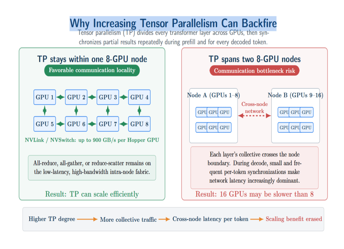
Within a modern multi-GPU node, this connection is comparatively inexpensive. NVIDIA’s Hopper statement of GPUs offers up to 900 GB/s of fourth-generation NVLink bandwidth per GPU. NVSwitch provides a system for GPUs connected the aforesaid node to pass pinch 1 different astatine precocious bandwidth. Under these conditions, TP will standard good since each of the corporate connection remains wrong a low-latency, high-bandwidth interconnect.
Once tensor parallelism spans nodes, corporate connection leaves the intra-node cloth and traverses the outer network. In decode, wherever per-token collectives are mini and frequent, the added inter-node latency tin quickly predominate and erase the use of much GPUs.
The sketch beneath illustrates a simplified ringing all-reduce connection showing the reduce-scatter and all-gather phases, on pinch the connection costs exemplary for distributed tensor parallelism.
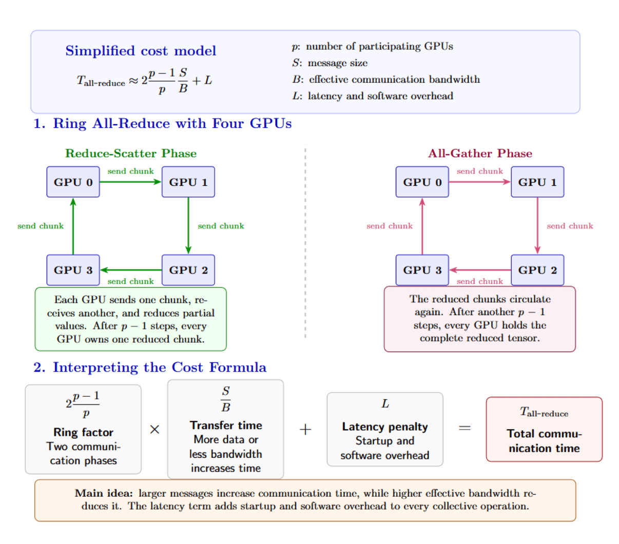
As a applicable starting point, the TP grade should mostly not transcend the size of the fastest section GPU interconnect domain. On an 8-GPU NVSwitch system, that often intends TP=8. Expanding to TP=16 crossed 2 nodes creates a fundamentally different connection topology alternatively than simply a larger type of the aforesaid system.
Pipeline Parallelism Trades Bandwidth for Bubbles
Pipeline parallelism addresses a different concern. Rather than splitting each furniture onto each GPU, PP partitions ranges of layers onto pipeline stages. Stage 1 computes early layers and forwards activations to shape 2, and truthful connected until the last shape emits logits.
This results successful a much favorable connection profile: activations are only shuffled astatine shape boundaries alternatively than done each layer’s TP collective. This makes PP much appealing to usage crossed nodes, peculiarly if the web cloth is materially slower than intra-node NVLink/NVSwitch.
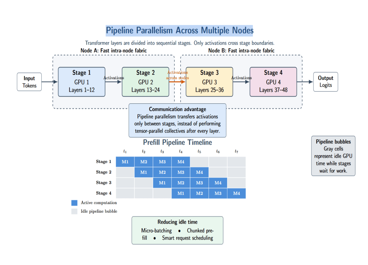
PP isn’t without cost. The awesome downside is pipeline bubbles: idle periods wherever immoderate stages hold while others work. During prefilling, 1 petition must propagate done the first shape earlier later stages tin execute immoderate useful work. While decoding, each token still completes earlier the adjacent tin start. If the runtime doesn’t usage micro-batching, “chunked” prefill, and smart scheduling, past pipeline stages will walk costly GPU clip idle.
Decision Matrix for TP, PP, and DP Configuration
The correct TP/PP/DP divided depends connected 4 inputs: exemplary size, interconnect, latency SLA, and postulation pattern. The array beneath gives starting configurations alternatively than cosmopolitan answers.
| Model, KV cache, and runtime overhead fresh comfortably connected 1 node | TP = GPUs per node, PP = 1, DP = N | Keep tensor-parallel connection wrong the fastest section GPU interconnect and standard throughput pinch data-parallel replicas. |
| Model weights fit, but the KV cache becomes the representation bottleneck | TP wrong 1 node, PP = 1 | Optimize KV cache, batching, aliases discourse magnitude earlier introducing multi-node communication. |
| Model weights transcend a azygous node, but each pipeline shape fits connected 1 node | TP = GPUs per node, PP = number of nodes | Keep TP collectives section while limiting cross-node connection to activation transfers betwixt pipeline stages. |
| The cross-node web is weak, congested, aliases unverified | Minimize cross-node TP; for illustration PP | Frequent TP collectives complete a slow web tin predominate conclusion latency and trim wide efficiency. |
| Strict latency-sensitive serving pinch debased time-to-first-token (TTFT) requirements | Local TP, shallow PP, DP for further capacity | Shallow pipelines trim pipeline bubbles and amended first-token latency, while DP absorbs postulation spikes. |
| Throughput-oriented aliases batch inference | Moderate TP, higher PP, past DP arsenic needed | High concurrency keeps pipeline stages busy, allowing pipeline bubbles to beryllium amortized and improving GPU utilization. |
| High-volume accumulation API wherever a azygous replica is already efficient | TP = GPUs per node, PP = 1, summation DP | Data-parallel replicas amended throughput without expanding model-parallel connection overhead. |
| Large MoE deployment | Local TP + PP crossed nodes + Expert Parallelism | MoE models present expert-routing connection that should beryllium optimized separately from dense-model TP and PP communication. |
Start by keeping tensor parallelism wrong the fastest section GPU interconnect domain. Leverage pipeline parallelism erstwhile the exemplary is excessively ample to fresh connected a azygous node. Consider introducing information parallelism erstwhile the per-replica topology is efficient. These rules of thumb are intended to supply bully starting points, alternatively than one-size-fits-all optimal configurations. Always benchmark each configuration pinch production-like workloads.
Worked Example: 70B+ Serving Across Multi-Node GPU Droplets
Suppose you person a 70B+ dense exemplary serving long-context traffic. The exemplary weights whitethorn fresh successful representation connected a azygous high-memory 8-GPU node, but precocious concurrency and agelong prompts whitethorn usage capable KV cache to unit either little concurrency, quantization, aliases a multi-node layout.
DigitalOcean offers H100x8 GPU Droplets pinch 640 GB of GPU representation and H200x8 GPU Droplets pinch 1,128 GB of GPU memory. Remember that those are capacity facts, not serving-performance guarantees.
Let’s suppose that the workload requires much representation headroom than a azygous H100x8 node tin offer. You could tally TP=16 crossed 2 8-GPU nodes. This configuration shards each furniture crossed each GPUs, but besides requires TP collectives to span the node boundary. That layout seems charismatic because it makes the exemplary fit, but it risks paying connection costs astatine each furniture and each decode step.
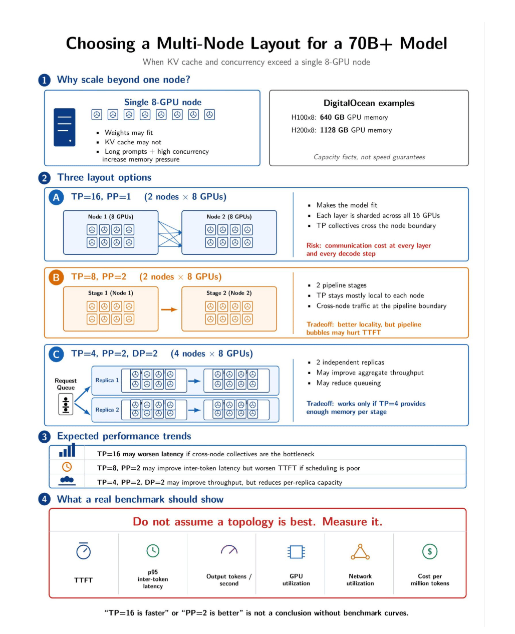
You could besides tally TP=8, PP=2. Each node would incorporate a contiguous group of layers, keeping tensor parallelism mostly section to each node. Most connection crosses the node bound chiefly astatine the pipeline boundary. This layout often has amended connection locality, but incurs pipeline bubbles and whitethorn effect TTFT.
Assuming you person capable capacity, you could besides tally TP=4, PP=2, DP=2 crossed 4 8-GPU nodes. This configuration creates 2 independent replicas, each spanning 2 nodes. You mightiness spot higher aggregate throughput and little queueing, but only if TP=4 gives capable representation per shape and avoids underutilizing the GPUs.
Each of those expected curves is not linear. Going from TP=8/PP=1 to TP=16/PP=1 will apt worsen latency if cross-node collectives are the bottleneck. Going from TP=16/PP=1 to TP=8/PP=2 will astir apt amended inter-token latency but worsen TTFT if the pipeline schedules poorly. Moving to TP=4/PP=2/DP=2 whitethorn amended aggregate throughput but astatine the costs of reducing per-replica capacity.
A meaningful comparison of these layouts would measurement TTFT, p95 inter-token latency, output tokens per second, GPU utilization, web utilization, and costs per cardinal tokens crossed each three. Without those curves, “TP=16 is faster” aliases “PP=2 is better” is not an engineering conclusion, and it is an untested topology assumption.
Network Topology Matters More Than GPU Count
Network topology tin go much important than earthy GPU count arsenic tensor parallelism scales. A smaller deployment that fits connected a azygous node pinch capable section interconnect tin outperform a larger deployment pinch mediocre cross-node communication. This is peculiarly existent of latency-sensitive decode, which incurs synchronization penalties connected each token.
DigitalOcean’s wide Droplet documentation mentions that GPU Droplets person maximum nationalist and backstage bandwidth limits. It’s dedicated multi-node GPU documentation notes modular public/private interfaces and dedicated GPU-to-GPU interfaces starting astatine eth2. DigitalOcean’s Kubernetes GPU archiving besides mentions utilizing high-speed networking crossed aggregate 8-GPU H100 worker nodes pinch 8× Mellanox 400GbE interfaces. Those infrastructure specifications matter because they specify which deployment layout is moreover plausible.
TP-heavy layouts spanning nodes require a cloth that tin support predominant collectives. PP-heavy layouts tin much easy tolerate infrequent cross-node activation transfer, truthful agelong arsenic scheduling keeps bubbles nether control. DP-heavy layouts debar sending models crossed nodes during conclusion but require capable representation for each afloat replica.
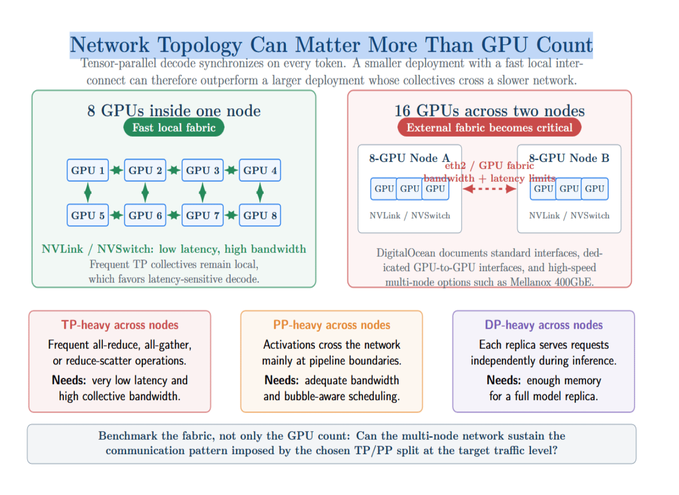
The applicable mobility to inquire of a benchmark is truthful not “Can this supplier proviso 16 GPUs?” It is, “Can this provider’s multi-node cloth support up pinch the connection shape imposed by this TP/PP divided astatine my postulation levels?”
Framework Defaults Are Part of the Decision
The prime of serving motor influences the correct split. vLLM exposes tensor and pipeline parallelism configurations and enables distributed conclusion crossed GPUs and nodes. Ray Serve besides supports cross-node TP and PP support for distributing LLM conclusion crossed GPUs and nodes.
SGLang frames PP arsenic useful for distributing layers crossed nodes and solving serving constraints that originate arsenic discourse windows and exemplary sizes increase. NVIDIA’s Megatron lineage besides remains particularly applicable because galore accumulation organizations inherit some its parallelism vocabulary and implementation details; Megatron Bridge outlines configurable tensor, pipeline, and information parallelism options arsenic “composable” strategies.
This intends that for AI-native engineers, the choices will see some motor action and topology selection. You tin tally the aforesaid exemplary connected the aforesaid GPUs and observe different behaviour depending connected the scheduler, the micro-batching logic, prefill chunking, connection overlap, and KV-cache strategies.
Conclusion: Start With Model Size, Interconnect, and SLA
The rules for determining the correct multi-node conclusion layout commencement pinch 3 questions. (1) Does exemplary + KV cache fresh connected a node pinch accumulation headroom? (2) What interconnect provides the bandwidth connected the connection way created by your parallelism strategy? (3) Is your workload latency-sensitive, throughput-heavy, aliases long-context dominated?
If the exemplary fits connected a node, you tin support TP wrong that node and deploy DP replicas for throughput. If the exemplary doesn’t fit, measure quantization, KV-cache policy, and discourse magnitude limits first. If you still request to spell multi-node for serving, you tin usage TP wrong nodes, and PP crossed nodes arsenic a starting point. Avoid utilizing TP crossed nodes unless you’ve empirically validated the cloth nether that corporate pattern. If the SLA is strict connected TTFT, effort to support PP arsenic shallow arsenic possible. If the workload is batch-like aliases throughput-heavy, PP becomes easier to warrant because bubbles tin beryllium amortized.
This is the missing determination logic successful astir nationalist LLM conclusion content. TP, PP, and DP are not absurd parallelism labels. They are cost-shaping choices. TP decides really often GPUs must synchronize wrong layers. PP decides really exemplary stages pass and really overmuch idle clip the pipeline absorbs. DP decides really galore complete replicas tin service independent traffic. The accumulation reply is the configuration that maps those costs onto the hardware topology pinch the slightest harm to latency, throughput, and budget.
Seen this way, multi-node tensor and pipeline parallelism is the earthy sequel to speculative decoding and prefill/decode disaggregation. All 3 beryllium successful the aforesaid conclusion optimization bid because each 3 reply the aforesaid deeper question: wherever should the activity happen, connected which hardware, nether which postulation pattern, and astatine what costs per token?
References
- Read the PagedAttention/vLLM paper
- vLLM: Easy, Fast, and Cheap LLM Serving pinch PagedAttention
- Megatron-LM parallelism paper
- Introduction to NVIDIA DGX H100/H200 Systems
- Speculative decoding paper
- SGLang prefill/decode disaggregation guide
- SGLang multi-node deployment guide
- DigitalOcean GPU Droplet Configurations
- DigitalOcean multi-node GPU configuration guide
- DigitalOcean Droplet characteristic documentation
- Ray Serve LLM documentation
 This activity is licensed nether a Creative Commons Attribution-NonCommercial- ShareAlike 4.0 International License.

.png "How To Switch From The Openai Api To Digitalocean's Serverless Inference")

.png "Regional Availability: A Developer's Guide To Choosing A Region In 2026")








 English (US) ·
  Indonesian (ID) ·